This section will provide a very brief overview of Apache Spark.

Spark is a product of the very prolific Berkeley AMP lab and it is now available everywhere.    On Amazon’s cloud it is available as part of their Elastic Map Reduce service.  On Azure it is part of HDInsight.  In both cases it runs on top of the Hadoop Distributed file system.   Spark is also easy to deploy as a Docker container on a single multicore Virtual machine.   It is also packaged as part of the Azure Data Science VM.

Spark is a cluster data analysis engine that consist of a master server and a collection of workers. A central concept in Spark is the notion of a Resilient Distributed Dataset (RDD) which represents a data collection that is distributed across servers and mapped to disk or memory. Spark is implemented in Scala which is an interpreted statically typed object functional language.   Spark has a library of Scala “parallel” operators that perform transformations on RDDs.   This library also has a very nice Python binding.   These operators are very similar to the Map and Reduce operations that were made popular by the Hadoop data analysis engine.   More precisely Spark has two types of operations: transformations which map RDDs into new RDDs and actions which return values back to the main program (usually the read-eval-print-loop).

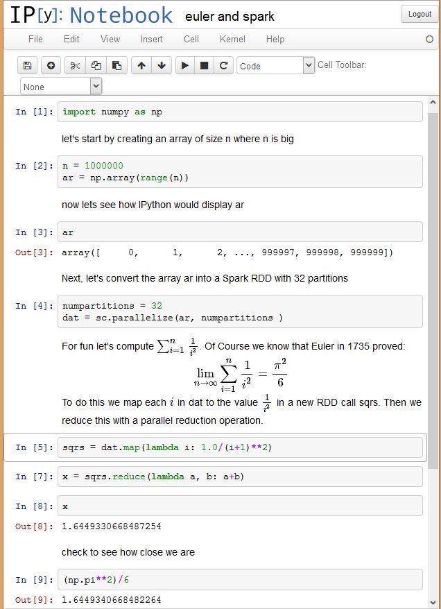
To illustrate these ideas look below at a sample from an IPython notebook session using Spark. In this example we create a one dimensional array of integers and then we convert this to an RDD that is partitioned into 32 pieces.   In Spark the partitions are distributed to the workers. Parallelism is achieved by applying the computational parts of Spark operators on partitions in parallel using workers and multiple threads per worker.   For actions, such as a reduce, most of the work is done on each partition and then across partitions as needed.   The Spark python library exploits the way Python can create anonymous functions using the lambda operator.   Code is generated for these function and they can then be shipped by Spark’s work scheduler to the workers for execution on each RDD partition.   If you have not seen the Notebook prior to this, it is fairly easy to understand. You type commands into the cells and then evaluate them. The commands may be Python expressions or they may be Markdown or HTML text including Latex math.   This combination of capabilities defines how the notebook can be used.   One can execute a Spark or Python command then make a note about the result. You can then go back to a previous step and change a parameter and rerun the computation. Of course, this does not capture the full range of data provenance challenges that are important for science today, it is a great step towards producing an executable document that can be shared and repeated. (If the image below is fuzzy, just click on it..)

Let me go through another simple example adapted from the Spark demo examples.  This is the one referenced in the main blog.  I have a large file of (x, y) coordinate pairs representing points randomly generated in an annular region around a circle of radius 10. There is one (x, y) pair per line of text.   In the first two lines in the figure below i define a RDD called lines that represents the lines of the text. To create an RDD one uses the “Spark Context” object sc that is already loaded into your notebook session. Using the textFile member function of sc I have provided the path to my file. I have specified that the RDD contains 8 partitions. That means that if n is the number of lines in the file, n/8 lines are in each partition. (In this case n happens to be about 95 million).   In the third line we create a new RDD called data which represents an n by 2 array of floating point numbers that are created by apply the function parseVector to each line of text. parseVector takes a line of text and returns the two numbers contained in the line. We also state that we want that RDD “cached” so that it can be reused later.   Note that the data RDD will also have the same number of partitions as lines.

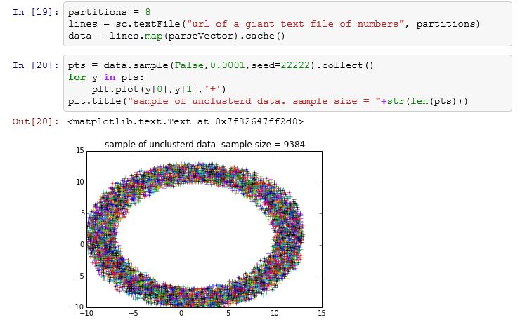
Up to this point no actual computation has taken place. Spark is lazy! (A computer science technical term that means don’t do any computation until it is really needed.) So far these operations have been transformations.   In the second block of code we encounter actions and real work must get done.   In this case we want to see what this data set looks like, but we don’t want to plot nearly 100 million points.   So we apply another transformation and generate a random sample of 0.0001 of the data points.   The real action happens when we want to “collect()” that sample and return it to the IPython notebook as an array of size 9384 x,y pairs. To execute the collect all of the previous transformations must be done so that we can create the array pts that we will plot.
Now that we have the big RDD data and it is cached we can apply additional trasformations. The Spark tutorial has a great example of a very elegant implementation of the KMeans clustering algorithm. This code is shown in the figure below.  (click on the figure to enlarge.)

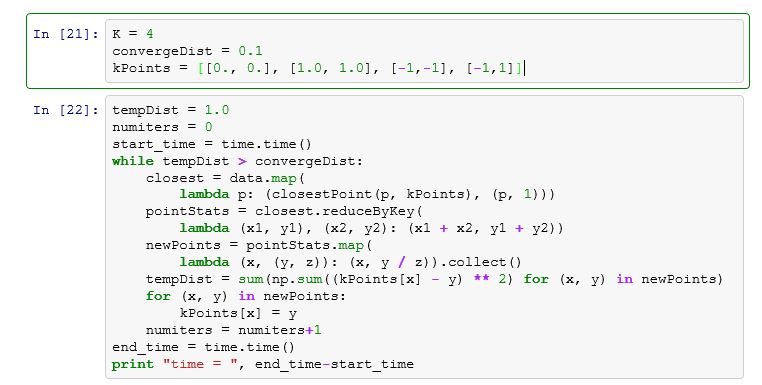
Without going into too many details of how this works, it is worth noting the structure of the program. There is an outer loop that measures the convergence of the algorithm.   Inside the loop we have two new RDD created. To do the computation Spark creates anonymous functions from lambda expressions. Code for these functions is generated and sent to each of the workers holding partitions of the RDD in question. The array kPoints hold the current guess of the centroids of the four clusters we are looking for.   The RDD closest is a set of (k, (p, 1)) for each point p in data where k is the index in kPoints in of the centroid closest to p. In the second step we reduce this set into four tuples (k, (sum of p in near kPoints[k], total number near kPoints[k])) for k = 0,1,2,3.   We can then compute new centroid by computing the mean (sum/total) of the points near kPoint[k]. TempDist measures the amount we have moved the centroids. If this is small, we stop.

We discuss the results of testing this program in the blog.  Note that the blog is old and it was carried out using a deployment “Brisk” that may no longer be available, the same Spark code runs on any of the spark deployments mentioned at the top of this page.