In this post we explore the IPython notebook on Azure via Elastacloud’s new Brisk Spark Service. We also look at Spark’s parallel scalability performance using a simple example.

Data analytics is about data exploration and that is an activity that is best done interactively. By interactive exploration we mean the ability to load a dataset into a system and then conduct experiments with different transformations and visualizations of the data. Interactive systems allow you to apply different analysis or machine learning algorithms and then experiment with different parameters to optimize the results. We have had great desktop tools for interactive data analysis for many years. Excel, Matlab, R, Mathematica are all superb in that they integrate a great computational library with graphics.   Mathematica demonstrated the power of journaling data exploration with an interactive electronic notebook. And the Scientific Python community has rallied around the IPython notebook.  This notebook is actually a web server that allows your browser to host the notebook files that you can interact with while Python runs in the background.   The good folks at Continuum Analytics provide the Anaconda package that contains all you need to deploy the Python, IPython, the scientific libraries including numpy, scipy and scikit-learn and the IPython notebook.   It is trivial to run the notebook on your laptop and interactively build and visualize python data analysis solutions. Individual notebooks can be published and shared with the notebook viewer nbviewer.

There is a major limitation to these desktop computing solutions. They are limited to the computing power and data capacity of your personal machine.   “Big Data” is a term that is frequently used without a precise definition.   I believe there is a very reasonable translation.   “Big Data” means too big to fit on your laptop. And the way you handle big data is to distribute it over multiple compute and storage nodes where you can apply parallel algorithms to the analysis.

If you have a supercomputer, you can submit batch analysis jobs, but if you want an interactive experience you must have a way for the user to submit individual commands to be executed followed by a response from the machine before another command is sent. This pattern is called a “read-eval-print-loop”, or REPL and the idea is as old as the hills. But for big data problems you need to do this with the user at a web browser or desktop app communicating with a massively parallel analysis engine in the back end. This has been done using Matlab clustering and the IPython notebook has a built-in parallel cluster tool.   More recently there is great interest in Torch and the LuaJIT programming environment. Torch is extremely strong in machine learning algorithms and exploits GPU parallelism with an underlying C/CUDA implementation.

Spark with IPython Notebook.

In this blog I want to talk about my experience using the IPython Notebook with the Spark analysis framework. Using the IPython notebook with Spark is not new. Cloudera described this in a blog post in August of 2014 and it is described in the Spark distribution. My goal here is to talk about how it fairs as an interactive tool for data analysis that is also scalable as a parallel computing platform for big data.

Spark is a product of the very prolific Berkeley AMP lab. It is now supported by Databricks.com who also provide an on-line service that allows you to deploy an instance of Spark on an Amazon AWS cluster. The Databricks Workspace contains a notebook that support SQL, Scala (the implementation language for Spark) and IPython. This same workspace also includes a way to transform a notebook into an online dashboard with only a few mouse clicks. This is an extremely impressive tool. Databricks is not the only company to make Spark a cloud service. The U.K. company Elastacloud has produced a new Brisk service that provides Spark on Microsoft’s Azure cloud. I will focus my discussion on experience with Brisk and a simple deployment of Spark on a 16 core Azure Linux VM server.

I describe Spark in greater detail in another section, however a brief introduction will be important for what follows.   Spark is a cluster data analysis engine that consist of a master server and a collection of workers. A central concept in Spark is the notion of a Resilient Distributed Dataset (RDD) which represents a data collection that is distributed across servers and mapped to disk or memory. Spark is implemented in Scala which is an interpreted statically typed object functional language.   Spark has a library of Scala “parallel” operators that perform transformations on RDDs.   This library also has a very nice Python binding.   These operators are very similar to the Map and Reduce operations that were made popular by the Hadoop data analysis engine.   More precisely Spark has two types of operations: transformations which map RDDs into new RDDs and actions which return values back to the main program (usually the read-eval-print-loop).

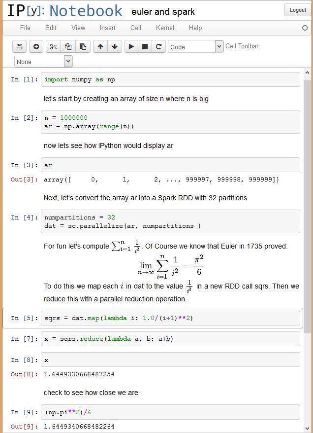
To illustrate these ideas look below at a sample from an IPython notebook session using Spark. In this example we create a one dimensional array of integers and then we convert this to an RDD that is partitioned into 32 pieces.   In Spark the partitions are distributed to the workers. Parallelism is achieved by applying the computational parts of Spark operators on partitions in parallel using workers and multiple threads per worker.   For actions, such as a reduce, most of the work is done on each partition and then across partitions as needed.   The Spark python library exploits the way Python can create anonymous functions using the lambda operator.   Code is generated for these function and they can then be shipped by Spark’s work scheduler to the workers for execution on each RDD partition.   If you have not seen the Notebook prior to this, it is fairly easy to understand. You type commands into the cells and then evaluate them. The commands may be Python expressions or they may be Markdown or HTML text including Latex math.   This combination of capabilities defines how the notebook can be used.   One can execute a Spark or Python command then make a note about the result. You can then go back to a previous step and change a parameter and rerun the computation. Of course, this does not capture the full range of data provenance challenges that are important for science today, it is a great step towards producing an executable document that can be shared and repeated.

Spark on Microsoft Azure

I deployed Spark with the IPython Notebook on Microsoft Azure in two different ways.   In the first case I took the standard spark 1.0 download, together with Anaconda and deployed it on an Azure D14 instance (16 cores, 112GB ram, 800 GB disk.)   This instance allowed me to test Spark’s ability to exploit threads in a multicore environment.   Spark is executed on a Java VM and threads in Java are used to execute the tasks that operate on partitions in an RDD.

The second deployment was made possible by the Elastacloud team and their new Brisk service.   Using Brisk one can create a spark cluster with on Azure with a few mouse clicks. The Azure usage is billed to your regular Azure accounts. Once your cluster has been created you are presented with a dashboard with links to important application monitoring tools.   I created small demo Spark cluster consisting of two nodes with four core each.   (In future posts I hope to have results for much larger clusters.)   After logging on to the head node I was able to install the IPython notebook with about a dozen steps.   (The Elastacloud people are considering the addition of the notebook as part of their standard package in a future release, so a separate installation will not be necessary.)

How Scalable is Spark?

To answer this question I set up a notebook that contained the standard Spark Python demo implementation of the KMeans clustering.   This is a very elegant, simple demonstration of a loop nest of data parallel operations. It is not the optimized version of KMeans in the latest release of MLlib for Spark. I am using this demo because we have all aspects of its implementation at hand. I will describe the details of the computation in another page.   I measured the performance across four data sets each consisting of n points randomly chosen in an annular band around the origin in 2D space.   The values of n for each of the data sets were 100,000, 1,000,000, 10,000,000 and 100,000,000 respectively.

First a few caveats. Doing KMeans on a set of 100 million 2D points could seldom be considered a really useful operation. But as a simple test of a systems scalability we can learn a few things.   It is also important to ask how does Spark compare to the best I can do on my desktop machine? (In my case a mid-sized windows laptop.) So I wrote a small program that used the nicely optimized Scikit-Learn version of KMeans.   I ran it against the same data.   The results were as follows.   Scikit-Learn was over 20 times faster than the naïve demo implementation of KMeans for the two smaller data sets! But the desktop version could not even load and parse the big files in a reasonable amount of time.   So by my earlier definition, these qualify as “big data”.

Scalability really refers to two dimensional properties of a system and an application.   One dimension relates to how the application performs as you increase the available parallel resources.  The other dimension is how the application performs as you increase the size of the problem it must solve. These things are related as we will show below.

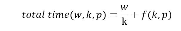
There are really two parameters that increase opportunities for parallel computation in Spark.   One is the total number of available cpu cores and how they are distributed over worker servers.   The other parameter is how we have partitioned the RDDs.   If we let k be the number of partitions of the data and let W be the amount of total time needed to execute the program when k = 1. If k is less than the number of available cores to do the computation and if the work divides up perfectly, the time to complete the execution will be W/k. This assumes that one cpu core is available do to the computation on each of the k partitions. However, work does not divide up perfectly. Reduction operations require data shuffling between workers and task scheduling overhead increase as k increases.   If we assume that overhead is a function of k and the number of available cores p, f(k,p), then the total time will be

We can then ask about the idea speed-up: the factor of performance improvement from one partition to k.

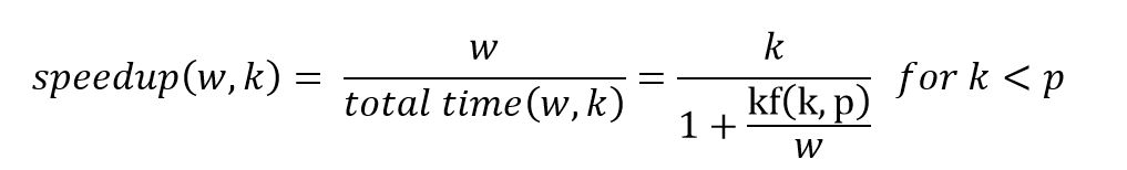
But this formula is only a rough guide as it does not factor many other system variables.   However, it does tell us that as w grows to be much larger than kf(k,p) then for k < p we can expect approximately linear speed up with the number of partitions.  As k grows bigger than p we expect that the speedup will be bounded above by p. A factor not accounted for here is opportunistic scheduling or more efficient use of cache when the size of each partition becomes smaller. Hence it is possible that for some k > p, the speedup will continue to grow. In the plot below we show the speedup behavior on our 16 core Azure server. There are two lines: the top represents the performance of our KMeans on the one million point dataset where the number of partitions of the data is on the x-axis. The line below is the performance on the 100K dataset.   These numbers represent averages for a small number of tests, so there is little statistical significance, but it is worth noticing three things.

• Both data sets reach a maximum speedup near 16 partitions which is equal to the number of cores and by the time you reach 32 partitions the overhead is dragging down performance.
• For the 1M point dataset the speedup exceeds k for k=2, 4 and 8.   This may represent more efficient scheduling behavior due to the smaller size of the partitions.
• The 16 core server was unable to complete the execution of the 10M data set size because the java heap size limits were exceeded.   (I was unable to figure out how to set it larger.)

The bottom line is that we do see scalability as the size of the problem grows (up to the heap size limit) and as we adjust the number of partitions.

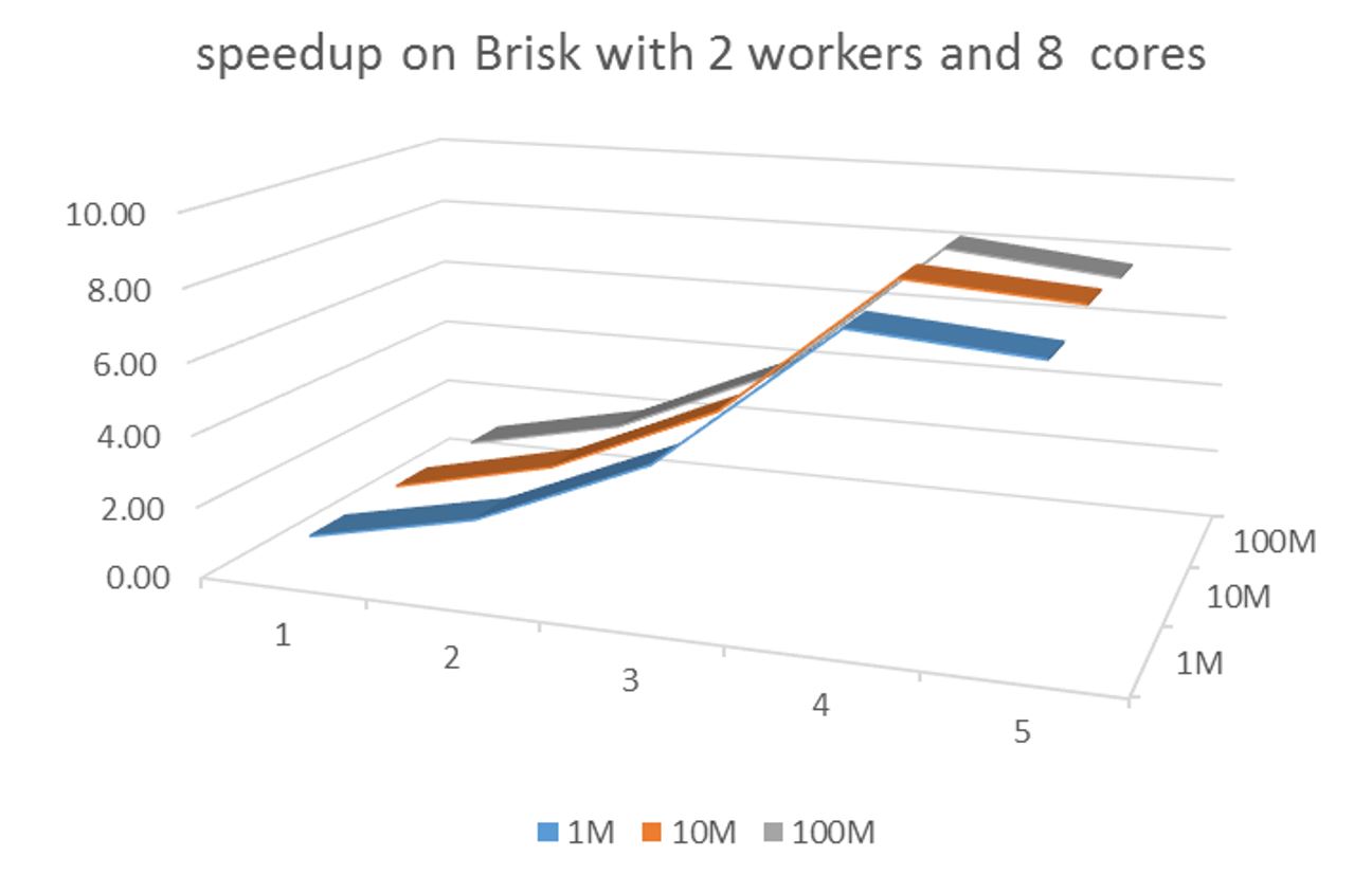
On the Brisk implementation we see greater scalability due to the fact that it is a cluster implementation.  The Brisk implementation was able to handle the 1M, 10M and 100M data set sizes while the total core count was only 8.   The maximum speed-up was around 8 and that was achieved with 16 partitions. In fact, the speedup curves were so close to each other they could not be plotted in 2D.

Additional Comments

The experiments described above do not constitute a proper scientific analysis, but they were enough to convince me that Spark is a scalable system that works well as a back end to the iPython notebook.   But there are several areas where much more needs to be done.   First, the size of these deployments are extremely small.   A proper study should involve at least 32 workers with 4 to 8 cores each. Second, these tests would be much better with optimized versions of the algorithms.