In a previous post we described Algorithmia,  a cloud service for discovering, invoking and deploying algorithms.  In this short article we look at Algorithmia as a tool to deploy trained machine learning models.   We used a tool called Gensim to build a model of scientific documents and then create an Algorithmia service that uses the model to predict the topic categories of scientific article.

A Review of Word Vectors and Document Vectors.

This technology has been around for a while now, so this review is more of a history lesson and not a deep technical review.  However, we will give you links to some of the important papers on the subject.

If you want to do document analysis through machine learning, you need a way to represent words in a vector form.  Given a collection of documents you can extract all the words to create a vocabulary.  If the size of the vocabulary is 100,000 words, you can represent each word as a “one-shot” vector in which the i-th word in the vocabulary is a vector of zeros except for a 1 in the i-th position.   Then if your then each document in your collection can be represented as the sum of vectors corresponding the words in that document.   If you have M documents, then the collection is represented by the sparse matrix of size M x 100,000.  Using this “bag of words” representation, there are a variety of traditional techniques such as Latent Sematic Analysis that can be used to extract the similarities between documents.

About five years ago, a team from Google found a much better way to create vectors from words so that words that are used in similar semantic context are nearer to each other as vectors.   Described in the paper by Tomas Mikolov et. all.,  the method, often referred to as Word2Vec, can be considered a map m() of our 100,000 dimension space of word to a dense space of much smaller dimension, say 50, with some remarkable properties.   In particular, there is the now-famous analogy linearity relationships. For example “man is to king as woman is to queen” is expressible (approximately) as

m( king) – m(man) + m(woman)   ≈   m(queen)

There is an excellent set of technical explanations of why Word2Vec work on Quora and we won’t go into them here.  One of the best papers that address this issue is by Golberg and Levy.

Le and Mikolov have shown that the basic methods of Word2Vec generalized to paragraphs, so that we now have a map p() from a corpus of paragraphs to vectors. In other words, given a corpus of documents D of size N, then for any doc d in D, p(d) is a vector of some prespecified length that “encodes” d.  At the risk of greatly oversimplifying, the paragraph vector is a concatenation of a component that is specific to the paragraph’s ID with word vectors sampled from the paragraph.   (As with Word2Vec, there are actually two main versions of this model.  Refer to the Le and Mikolov paper for details.)  It turns out that the function p can be extended to arbitrary documents x so that p(x) is an “inferred” vector in the same space vector space.  We can then use p(x) to find the documents d such that p(d) is nearest to p(x).      If we know how to classify the nearby documents, we can make a guess at the classification of x.  That is what we will do below.

Using Doc2Vec to Build a Document Classifier

Next we will use a version of the Paragraph vectors from Gensim’s Doc2Vec model building tools and show how we can use it to build a simple document classifier.  Gensim is a product of  Radim Řehůřek’s RaRe Technologies.    An excellent tutorial for Gensim is this notebook from RaRe.  To initialize Gensim Doc2vec we do the following.

import gensim
model = gensim.models.doc2vec.Doc2Vec(size=50, min_count=2, iter=55)

This creates a model that, when trained will have vectors of length 50.  The training will use 2 word minimum from each doc for each iteration and there will be 55 iterations.

Next we need to ready a document corpus.   What we will use is 7000 science journal article abstracts from the Cornell University archive ArXiv.org . We have recorded the titles, abstracts and the topic classifications assigned by the authors.   There are several dozen topic categories but we partition them into five major topics: physics, math, computer science, biology and finance.      We have randomly selected 5000 for the training set and we use the remainder plus another 500 from recently posted papers for testing.  We must first convert the text of the abstracts into the format needed by Doc2Vec.  The files are “sciml_train” and “sciml_test”.   The function below preprocesses each of the document abstracts to create the correct corpus.

def read_corpus(fname, tokens_only=False):
        with smart_open.smart_open(fname, encoding="iso-8859-1") as f:
             for i, line in enumerate(f):
                   doc = gensim.utils.simple_preprocess(line)
                   if tokens_only:
                       yield doc
                   else:
                       # For training data, add tags
                       yield gensim.models.doc2vec.TaggedDocument(d, [i])
train_corpus = list(read_corpus("sciml_train"))
test_corpus = list(read_corpus("sciml_test", tokens_only=True))

We next build a vocabulary from the words in the training corpus.   This is a dictionary of all the words together with the counts of the word occurrences.  Once that is done we can train the model.

model.build_vocab(train_corpus)
model.train(train_corpus, total_examples=model.corpus_count, epochs=model.iter)

The training takes about 1 minutes and a simple 4-core server. We can now save the model so that it can be restored for use later with the Python statement model.save(“gensim_model”). We will use this later when building the version we will install in Algorithmia.
The model object contains the 5000 vectors of length 50 that encode our documents. To build our simple classifier we will extract this into an array mar of size 5000 by 50 and normalize each vector to be of unit length. (The normalization will simplify our later computations.)

import Numpy as np
mar = np.zeros((model.docvecs.count, 50))
for i in range(m.count):
    x = np.linalg.norm(model.docvecs[i])
    mar[i] = model.docvecs[i]/x

An interesting thing to do with the mar matrix is to visualize it in 2-d using the t-distributed stochastic neighbor embedding (t-SNE) algorithm. The result is shown in the figure below. The points have been color coded based on topic: 1(dee purple) = “math”, 2(blue gray) = “Physics”, 3(blue green) = “bio”, 4(green) = “finance” and 5(yellow) = “compsci”.

There are two things to note here.   First, the collection is not well balanced in terms of numerical distribution.  About half the collect is physics and there are only a small number of bio and finance papers.   That is the nature of academic science:  lots of physicists publishing papers and not so many quantitative finance or quantitative bio papers in the open literature.   It is interesting to note that the Physics papers divide clearly into two or  three clouds.  (it turns out these separate clouds could be classed as “astrophysics”  and “other physics”.)  Computer science and math have a big overlap and bio has a strong overlap with cs because these are all “quantitative bio” papers.

The classification algorithm is very simple. Our model has a function infer_vector(doc) that will use stochastic methods to interpret the doc into the model vector space. Using that inferred vector we can compute the nearest k documents to it in the model space with the function below.

def find_best(k, abstract):
	preproc = gensim.utils.simple_preprocess(abstract)
	v = model.infer_vector(preproc)
       v0 = v/np.linalg.norm(v)
	norms = []
 	for i in range(5000):
     		norms.append([np.dot(v0,mar[i]), i])
       return norms[0:k]

The dot product of the two normalized vectors is the cosine distance. Because the infer_vector is stochastic in nature, our final version of the classifier calls the find_best ten times and computes an average ranking. (The details are in this notebook. and an Html version.) Selecting one of the more recent abstracts and subjecting it to the classifier gives the result pictured below.

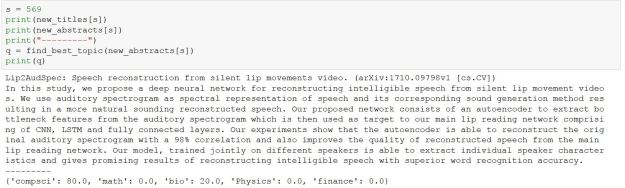
The analysis gives the abstract a score of 80 for computer science and 20 for bio. Note that the title contains the detailed ArXiv category, so we see this is correct, but reading the article it could also be cross listed as bio.
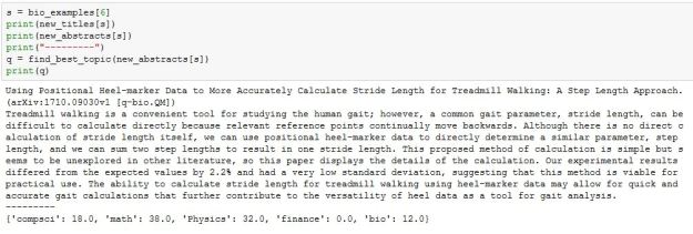
On the other hand, there are many examples that easily confuse the system. For example, the one below is classified as quantitative biology in arXiv, but the system can’t decide if it is math, cs or physics.

In general we can take the highest ranking score for each member of the test set and then compute a confusion matrix.  The result is shown below.  Each row of the table represents the percent of the best guesses from the system for the row label.

One interesting observation here is that in the cases where there is an error in the first guess, the most common mistake was to classify an abstract as mathematics.

Moving the model to Algorithmia

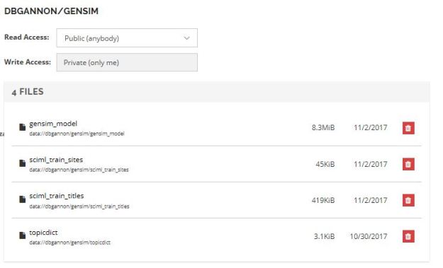
Moving the model to Algorithmia is surprisingly simple.  The first step is to create a data collection in the Algorithmia data cloud.   We created one called “gensim” and it contains the three important files: the gensim model,  topicdict, the dictionary that translates ArXiv topics to our major topics, and the ArXiv topics associated with each of the training documents.   The Algorithmia collection is shown below.  We also loaded the training document titles but they are not necessary.

The main difference between running a trained model in Algorithmia and that of a “normal” algorithm is the part where you load the model from the data container.   The skeleton of the python code now includes a function load_model()which you write and a line that invokes this function as shown below.  Now when your algorithm is loaded into the microservice it first calls the load_model()before invoking the apply(input) function.   For all subsequent invocations of you algorithm while it running in that microservice instance the model is already loaded. (The full source code is here. )

import Algorithmia
import gensim
From gensim.models.doc2vec import Doc2Vec
client = Algorithmia.client()
def load_model():
    file_path = 'data://dbgannon/gensim/gensim_model'
    file_path = client.file(file_path).getFile().name
    model = Doc2Vec.load(file_path)
    # similarly load train_sites and topicdict
    # and create mar by normalizing model data
    return model, mar, topicdict, train_sites

model, mar, topicdict, train_sites = load_model()
def find_best_topic(abstract):
    #body of find_best_topic
def apply(input):
    out = find_best_topic(input)
    return out

Deploying the algorithm follows the same procedure as before.   We add the new algorithm from the Algorithmia portal and clone it.   Assuming the SciDocClassifier.py contains our final version of the source,  we execute the following commands.

git add SciDocClassifier.py
git commit -m "second commit"
git push origin master

Returning to the Algorithmia portal, we can go to the project source editor. From there we need to add the code dependencies. In this case, we wanted exactly the same versions of gensim and Numpy we used in our development environment. As shown below that was easy to specify.

The final version has been published as dbgannon/SciDocClassifer and is available for anyone to use.  Once again, our experience with using Algorithmia’s tools have been easy to use and fun to experiment with. There are many algorithms to try out and a starter free account is all you need.