The Microsoft Azure team has recently released CosmosDB, an new entry to the cloud data storage management marketplace. Cosmos is actually the name of a data storage system that has been used internal to Microsoft for many years. That original Cosmos has now morphed into Azure Data Lake Storage (ADLS) and Analytics. ADLS is focused on Hadoop/HDFS compatible scalable analytics and, at the present time, it is available in only two of the US data centers. CosmosDB is related to the original Cosmos in name only and it is available at all of the data centers.

There is an excellent technical description [https://azure.microsoft.com/en-us/blog/a-technical-overview-of-azure-cosmos-db], so we will hit only a few highlights here.  CosmosDB has four main API components and a number of interesting properties. From the user’s perspective these components are

1. DocumentDB; “a NoSQL document database service designed from the ground up to natively support JSON and JavaScript directly inside the database engine.”
2. MongoDB; CosmosDB implements the MongoDB API so that users of that popular NoSQL database can easily move to CosmosDB.
3. Azure Table Storage: a simple key-value table mechanism that has been part of Azure from it earliest days.
4. Gremlin Graph Query API; a graph traversal language based on functional programming concepts.

There is a common “resource model” that unifies all of these capabilities. A database consists of users with varying permissions and containers. A container holds one of the three content types, document collection, tables or graphs. Special resources like stored procedures, triggers and user-defined-functions (UDFs) are also stored within the container. At the top level the user creates a cosmosDB database account and in doing so the user must pick one of these four APIs. In the examples we show here we focus on the DocumentDB API. In a later post we will look at Gremlin.

There are four important properties that every CosmosDB databased has.

1. Global distribution: your database is replicated in any of 30+ different regions and you can pick these from a map on the Azure portal.
2. Elastic scale-out: you can scale throughput of a container by programmatically provisioning throughput at a second or minute granularity. provision throughput (measured in using a currency unit called, Request Unit or RU).
3. Guaranteed low latency: For a typical 1KB item, Azure Cosmos DB guarantees end-to-end latency of reads under 10ms and indexed writes under 15ms at the 99th percentile within the same Azure region.
4. Five consistency models.
5. A Comprehensive Service Level Agreement (SLA).

Global Distribution

CosmosDB has two forms of distribution. Each database is composed of one or more collections and every data collection is stored in a logical container that is distributed over one or more physical server partitions. And, of course, everything is replicated. Every item in a collection has a partition key and a unique ID. The partition key is hashed and the hash is used to make the assignment of that item to one of the physical servers associated with that container. This level of partitioning happens automatically when you create a collection and start filling it.

Global distribution is more interesting. When you first create a database it has an initial “write location” which refers to one of the 30 or so Azure regions around the globe. You can use the portal to say how your data is distributed to other regions. In the example we discuss at the end of this document our original region “North Central US”. We have used the “Replicate Data Globally” function, which gives us a map in the portal, where we selected three additional regions, “West Europe”, “South India” and “Brazil South” as shown in Figure 1 below.

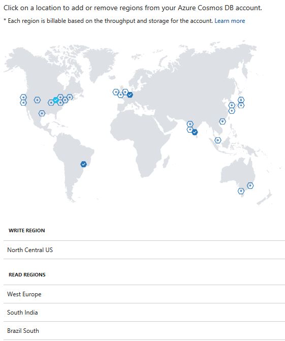
Figure 1. Selecting three additional locations for a database using a map tool.

With a small (170MB) database of documents it took only a few minutes to replicate the data to these locations. The data collections in the replicate sites are considered “read locations”. Which means that a user in these locations will by default read data from the local replica. However if that remote user attempts a write the request is routed to the “write location”. To understand how long a remote reader takes to see an update from the remote write location we need to discuss the consistency models.

Elastic scale-out and The Cost of Computing

Every operation you do in CosmosDB requires bandwidth and computation. You can control the rate at which “energy” is consumed for your database with something called Request Units (RU) and RUs/sec and RUs/min. You specify the RUs/sec you are willing to “spend” on your database and CosmosDB will provision the resources to meet your throughput requirements.

Consistency Models

Consistency is one of the most difficult topics in distributed systems. In the case of distrubted or replicated databases, consistency the consistency model tell the user how changes in one copy of a database are reflected updates to other copies. By insisting that consistency be very strong, this may have an adverse impact on latencies and throughput. So the choice of consistence model can have a profound impact on application performance and cost.

One of the truly unique features of CosmosDB is that it gives the user a choice of five different consistency models. In order from the weakest to the strongest and in terms of RUs, the cheapest to most expensive they are:

1. Eventual consistency. Eventual consistency is the weakest form of consistency wherein a client may get the values which are older than the ones it had seen before, over time. In the absence of any further writes, the replicas within the group will eventually converge.
2. Consistent prefix. Consistent prefix level guarantees that reads never see out of order writes. If writes were performed in the order `A, B, C`, then a client sees either `A`, `A,B`, or `A,B,C`, but never out of order like `A,C` or `B,A,C`.
3. Session consistency. When you connect to a cosmosDB database through its URL you are creating a session. Session consistency guarantees monotonic reads, monotonic writes, and read your own writes (RYW) guarantees for the duration of the session. In the Python API you create client object that encapsulates your connection to the database. The parameter “Consistency_level” has the default value “Session”. Reads in session consistency take a bit longer than consistent prefix which takes longer than eventual consistency.
4. Bounded stateness. This model has two ways to insist on consistency. You can define a time interval such that beyond that interval of time from the present, the system will guarantee consistency. Alternatively you can specify a the upper bound on the number of reads that lag behind writes your reader can be. Beyond that point consistency is guaranteed. Of course the smaller you make the window, the more computing you may consume and delay you may encounter.
5. Strong consistency. The most expensive and most complete. it is linearizable in that reads always returns the most recent writes. But it is limited to collections that are not geodistributed.

A word about the performance of these models. In the example at the end of this section we put the write region of the database in North America and replicated in three other locations with one in Western Europe. We then created a virtual machine in Western Europe and connected it to the database and verified by the IP address that it was connecting to the local replica. We then fired changes at the North America region and read with each of the consistency models. We were unable to detect any out of order reads and the responses were extremely fast. This is obviously not a full scientific study, but it was clear we had a system that performed very well. We also attempted a write to the local Western Europe “read location”. We were able to detect that the API call immediately dropped the read location connection and reconnected to the North American copy to do the write.

Comprehensive SLA

The service level agreement (SLA) for CosmosDB is actually a contract that Azure and you agree to when you create a database. It is indeed comprehensive. It covers guarantees for availability, throughput, consistency and latency giving you upper bounds for each measurable attribute of performance. As you are the one to specify how many RUs/sec you are willing to allocate, some of the temporal guarantees may be dependent upon this allocation not being exceeded. We will not go into it in detail here. Read it with your lawyer.

A look at Azure DocumentDB using Python and GDELT Data

To illustrate the basics of DocumentDB we will use a tiny part of the amazing GDELT event collection. This data collection is available on AWS S3 as well as Google’s BigQuery. The GDELT project (http://gdeltproject.org) is the brainchild of Kalev Leetaru from Georgetown University and it is an serious “Big Data” collection. GDELT’s collection is the result of mining of hundreds of thousands of broadcast print and online new sources from every corner of the world every day. What we will look at here is a microscopic window into the daily collection of news items. In fact, we will take a look at the news from from one day: June 30, 2017.

AWS keeps the data on S3 and downloading it is dead easy. The command

$ aws s3 cp s3://gdelt-open-data/events/20170630.export.csv . 

will download the 20MB June 30 2017 dataset as a CSV file. Each row of the file is a record of an “event” consisting of some 60 attributes that catalog a publication of a news item. Among the fields in the record are a unique identifier, a timestamp and the name and geolocation of two “actors” that are part of the event. In addition, there is a url a published news item about the event. The actors are derived from the even. Actor1 is called an initiator of the event and actor2 is a recipient or victim of the event. These actors are usually represented by the names of the cities or countries associated with the actual actors.

For example the story “Qatar’s defense minister to visit Turkey amid base controversy” (http://jordantimes.com/news/local/qatar’s-defence-minister-visit-turkey-amid-base-controversy) appeared in the Jordan Times. It describes an event where the Qatar defense minister visited Turkey as Turkey resists pressure from Saudi Arabia, the United Arab Emirates, Egypt and Bahrain to close bases after the five other nations pressed sanctions agains Qatar on June 5. This URL appears three time in the database for June 30. In one case, actor1 is Doha Qatar and actor2 is Ankora Turkey. In the second case actor1 is Riyadh, Saudi Arabia actor2 is Turkey. In the third case actor1 and actor2 are both Riyadh. Though the identity of the actor cities is based on an automated analysis of the story, their may be three different stories to analyze. However, only one URL has been selected to represent all three.

For our purposes we will describe this as a single event that links the three cities, Doha, Ankora and Riyadh. Many researchers have used this GDELT data to do deep political and social analysis of the world we live in, but that goal is way beyond what we intend here. What we will try to do in this example is to use CosmosDB to graphically illustrate different ways we can represent the events of June 30 and the cities they impact.

Creating the DocumentDB from the CSV file.

We will begin by creating a simple document database where each document is the JSON record for one line of the CSV file. Actually we will only include the URL, the two actor cities and their geolocations. To begin we must connect you client program to the CosmosDB system.

We use Python and we assume that the documented tools have been installed.

#run this if documentdb is not installed
#!pip install pydocumentdb
import csv
import pydocumentdb;
import pydocumentdb.document_client as document_client

We next create the database and the collection. But first we need an Azure CosmosDB account and is best done on the Azure portal. One that is there you can retrieve the account key so that we can create the collection.
Our account is called bookdockdb and our database is called ‘db3’ and the new collection will be called ‘gdelt’.

config = { 
    'ENDPOINT': 'https://bookdocdb.documents.azure.com',
    'MASTERKEY': 'your db key here',
    'DOCUMENTDB_DATABASE': 'db3',
    'DOCUMENTDB_COLLECTION': 'gdelt'
};
#we create the database, but if it is already there the "CreateDatabase will fail"
#In that case, we can query for it. 
#this is handy because we can have more than one collection in  a given database.
try:
    db = client.CreateDatabase({ 'id': config['DOCUMENTDB_DATABASE'] }, )
except:
    db_id = config['DOCUMENTDB_DATABASE']
    db_query = "select * from r where r.id = '{0}'".format(db_id)
    db = list(client.QueryDatabases(db_query))[0]

Next we will create the collection. Again, we may already have the collection there, so we can add new items to an existing collection but we need a different method to retrieve the collection handle.

options = {
    'offerEnableRUPerMinuteThroughput': True,
    'offerVersion': "V2",
    'offerThroughput': 400
}
try:
    collection = client.CreateCollection(db['_self'], 
         { 'id': config['DOCUMENTDB_COLLECTION'] }, options)
except:
    collection = next((coll for coll in client.ReadCollections(db['_self']) \
         if coll['id']==config['DOCUMENTDB_COLLECTION']))

The next step is to read the CSV file and add the new documents to the database collection.
We are going to do this one line at a time and keep only the time stamps, actor cities and geolocations (latitude and longitude) and the associated URL. We will also keep a separate list of the URLs for later use.

url_list = []
with open('20170630.export.csv') as csvfile:
    readCSV = csv.reader(csvfile, delimiter='\t')
    for row in readCSV:
        url_list.append(row[57])
        document1 = client.CreateDocument(collection['_self'],
            { 
             'id': row[0],
             'time_stamp': row[1],
             'time_stamp2': row[4],
             'city0_lat': row[46],
             'city0_lon': row[47],
             'city0_name': row[43],
              'city1_lat': row[53],
              'city1_lon': row[54],
              'city1_name': row[50],
              'url': row[57] 
              }
            )

The next thing we will do is to look at the URLs that involve a large number of cities (because they are often more interesting). Because we have the geolocations of each city we can draw a map and link the cities associated with the URL.

To do this we need to remove all the duplicates in our URL list using a standard Python trick: convert the list to a set and then back to a list.

s = set(url_list)
url_list = list(s)

We next query the database collection to find the cities associated with each URL. The best way to do this in the cloud is a simple map-reduce operation where we map each record to a pair consisting of a URL and a list of cities. We then invoke a reduce-by-key function to reduce all pairs with the same key to a single pair with that key with all of the lists associated with that key concatenated.
If we were doing more than a single day’s worth of data, It would be worth bringing Spark into the picture and using that for the map-reduce step. Instead we will do it sequentially using a data base query for each URL. The following function accomplishes that task.

def get_cities_for_url(url):
    db_query = {'query':"select * from r where r.url = '{0}'".format(url) }
    options = {}
    options['enableCrossPartitionQuery'] = True
    options['maxItemCount'] = 1000
    q = client.QueryDocuments(collection['_self'], db_query, options)
    results = list(q)
    cities = []
    for x in results:
        if x['city1_name'] != '':
            cities.append(x['city1_name']+" lat="+x['city1_lat'] + ' lon='+x['city1_lon'])
        if x['city0_name'] != '':
            cities.append(x['city0_name']+" lat="+x['city0_lat'] + ' lon='+x['city0_lon'])
    city_set = set(cities)
    cities = list(city_set)
    return cities

The function returns a list of strings where each string is a city and its geolocation. We have used the matplotlib Basemap tools to render the most interesting sets of cities where we define “interesting” to be those URL sets with more than 5 cities. In this case we have only plotted a few hundred of the city clusters.

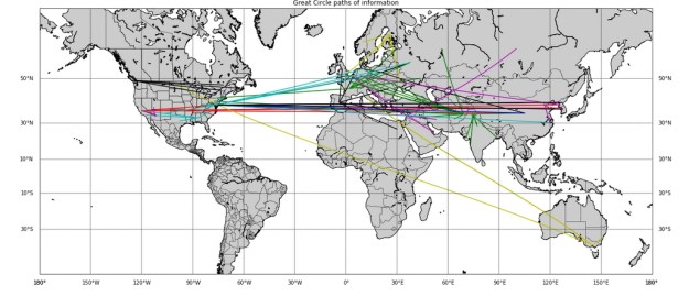
Figure 2.   Cities linked by shared stories.

While this is colorful, it is not very informative. We can tell there was some events in Australia that involved Europe and the US (this turned out to be a scandal involving an important person in the catholic church) and there was a number of stories that involve North Korea, the US and China. Something happened in the Northwest that involved cities in the east coast of the US.n general the information content is low.

To create a different view, let’s transform the collection to one that reflects the set of cities associated with each URL. To accomplish that we call the get_cities_for_url() function above and create a new document that only three attributes: an ID, the URL and a list of cities associated with the URL. The new collection is called “cities”, but it is really more like a dictionary that associates the URLs with a list of cities.  (The Jupyter Notebook used to build this collection and illustrate the example below is available here.)

One thing we can do is to search for special words or phrases in the URLs and list the cities that are associated. To do this we can make use of another feature of DocumentDB and create a user defined function to do the string search. This is extremely easy and can be done from the Azure Portal. The functions are all java script. The data explorer tab for the “cities” collection and select the “New User Defined Function” tab. In our case we create a function “findsubstring” that searches for a substring “sub” in a longer string “s”.

function  findsubstring(s, sub){
    t = s.indexOf(sub)
    return t
}

We can now call this function in a database query as follows.

def checkInDB(name):
    db_query = {'query':"select r.url, r.cities from r where udf.findsubstring(r.url,'{0}')>0".format(name) }
    options = {}
    options['enableCrossPartitionQuery'] = True
    options['maxItemCount'] = 10000
    q = client.QueryDocuments(collection['_self'], db_query, options)
    results = list(q)
    return results

Picking a name from the news, “Ivanka”, we can see what stories and cities mentioned “Ivanka” on that day. The call checkInDB(“Ivanka”) returns

[{'cities': ['Oregon, United States', 
'White House, District of Columbia, United States',
'Buhari, Kano, Nigeria',
'Canyonville Christian Academy, Oregon, United States ', 
'Chibok, Borno, Nigeria', 
'Virginia, United States'],
'url': 'http://www.ghanaweb.com/GhanaHomePage/world/Trump-and-Ivanka-host-two-Chibok-girls-at-the-White-House-553963'}]

which is a story about a reception for two girls that were rescued from the Boko Haram in Africa. The list of associated cities include Canyonville Christian Academy, a private boarding school that has offered to continue their education.

A More Interactive Abstract View of the Data.

Another interesting approach to looking at the data is to consider stories that link together smaller cities in some ways. We are going to look for “local” story connections rather than big news items. More specifically, we will look at cities that appear in at least 3 but no more than 5 stories in the days news. This leaves out big cities like washington DC and big global headlines. Next we will build a graph that we can use to explore the stories and cities that share these more regional stories. There are actually 245 cities that appear in our restricted set.

In order to make our graph we need a dictionary that maps cities into the list of stories that mention it. Call that dictionary “stories” Our visualization has nodes that are cities and we will connect them by an edge if they appear in a story together. Let “linkcities” be the list of 245 cities describe above. We can then compute the edges using as follows.

edges = []
for i in range(0, len(linkcities)):
    for j in range(0, len(linkcities)):
        if i < j:             
		iset = set(stories[linkcities[i]])             
		jset = set(stories[linkcities[j]])             
		kset = iset.intersection(jset)             
		if len(kset)> 0:
                	edges.append((i,j))

The complete code for this example is given in this Jupyter notebook. We use the Plotly package to build and interactive graph. The nodes are distributed approximately over the surface of a sphere in 3D. You can rotate the sphere and mouse over nodes Doing so, shows the URLs for the stories associated with that town. The sphere appears as the image below.

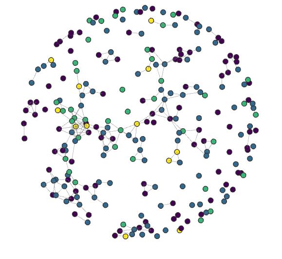
Figure 3.  Interactive city graph

A better way to see this is to interact with it. You can do this by going to the bottom panel in this file [https://SciEngCloud.github.io/city-graph.html].

Conclusion

Our experience with CosmosDB has been limited to using the DocumentDB API, but we were impressed with the experience. In particular, the ease with which one can globally distribute the data was impressive as were the selection of consistency protocols. As we said, we were unable to force the database to show temporary inconsistency even with the weakest protocol choice using very distant copies of the database. This should not be considered a fault. Our tests were too easy.  The examples above do not begin to stretch all the capabilities of CosmosDB, but we hope they provide a reasonable introduction for the Python programmer.)

One final comment. It seems CosmosDB was built on top of the Azure microservice container system. It would be very interesting to see more details of the implementation.