

Over the last five years cloud computing systems have evolved to be the home to more than racks of servers. The need for specialized resources to for various classes of customers has driven vendors to add GPU server configurations as a relatively standard offering. The rise of Deep Learning has seen the addition of special hardware to accelerate both the training and inference phases of machine learning. This include the Google Tensor Processing hardware in the Google cloud and the FPGA arrays on Microsoft’s Azure. Quantum computing has now moved from theory to reality. Rigetti, IBM, D-Wave and Alibaba now all now have live quantum computing services in the cloud. Google and Microsoft will follow soon. In the paragraphs that follow we will dive a bit deeper into several of these services with illustrations of how they can be programmed and used. In this article we will look at two different systems: the IBM-Q quantum computer and it software stack qiskit and the Microsoft Q# quantum software platform. We could have discussed Rigetti which is similar to IBM and D-Wave but it is sufficiently different from the others to consider it elsewhere. We don’t have enough information about Alibaba’s quantum project to discuss it.
The Most Basic Math
As our emphasis here will be on showing you what quantum programs look like, we will not go into the physics and quantum theory behind it, but it helps to have some background. This will be the shallowest of introductions. (You will learn just enough to impress people at a party as long as that party is not a gathering of scientists.) If you already know this stuff or you only want to see what the code looks like skip this section completely.
There are many good books that give excellent introductions to quantum computing. (My favorite is “Quantum Computing: A Gentle Introduction” by Rieffel and Polak.) We must begin with qubits: the basic unit of quantum information. The standard misconception is that it is a probabilistic version of a binary digit (bit). In fact, it is a two-dimensional object which is described as a complex linear combination of two basis vectors |0> and |1> defined as
 Using this basis, any qubit |Ψ> can be described as a linear combination (called a superposition) of these basis vectors
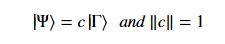
 where α and β are complex numbers whose square norms add up to 1. Because they are complex this means the real dimension of the space is 4 but then the vector is projected to complex projective space so that two qubit representatives |Ψ> and |г> are the same qubit if there is a complex number c such that
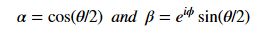
 A slightly less algebraic representation is to see the qubit |Ψ> as projected onto the sphere shown on the right
  where |Ψ> is defined by two angles where
Qubits are strange things that live in a world where we cannot know what the parameters α and β are unless we attempt to measure the qubit. Measurement can be thought of as projecting the qubit onto a special set of basis vectors and each device has its own set of basis vectors. Here we will assume all our measurements are with respect to the standard basis |0> and |1>. Measuring a qubit changes it and results in a classic bit 0 or 1. However, the probability that it is a 0 is || α ||2 and the probability we get a 1 is || β ||2. After a qubit has been measured it is projected into one of the basis vectors |0> and |1>.
Basic Qubit Operators
In addition to measurement, there are a number of operators that can transform qubits without doing too much damage to them. (As we shall see, in the real world, qubits are fragile. If you apply too many transformations, you can cause it to decohere: and it is no longer usable. But this depends upon the physical mechanism used to render the qubit.) The basic transformation on a single qubit can all be represented by 2×2 unitary matrices, but it is easy to just describe what the do to the basis vectors and extend that in the obvious way to linear combinations.
- X is the “not” transform. It takes |0> to |1> and |1> to |0>. By linearity then X applied to any qubit is

- H the Hadamard transform takes |0> to 1/√2(|0> + |1>) and |1> to 1/√2(|0> – |1>). This transform is used often in quantum programs to take an initial state such as |0> to a known mixed state (called superposition).
Multiple Qubits
Quantum computing gets interesting when multiple qubits interact. The way we describe the state space of two qubits is with the tensor product. For two qubits we can describe the state of the system in terms of the basis that is just the tensor product of 1-qubit basis:
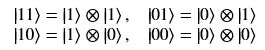
So that any state of the 2-qubit system can be describe as a linear combination of the form

For three qubits the eight basis elements are |000> through |111>. The real dimension of this 3 qubit space is 23= 8. There are deep mathematical reasons for why the tensor product is the correct formulation rather than the direct sum of vector spaces as in classical mechanics, but the result is profound. The real dimension of an n-qubit system is 2n. When n = 50 the amount of standard computer memory required to store a single qubit is 8*250 = 16 petabytes (assuming 2 8-byte floating point values per complex coefficient). Hence there are limits to the size of a quantum systems we can simulate on a classical computer. We now have functional quantum computers with 20 qubits and we can simulate 32 qubits, but it may take 50 qubits or more to establish the more promising advantages of quantum computing.
For two qubits there is a standard operation is often used. It is the
- Cnot Controlled Not. This operation is so called because it can be thought of as using the first qubit (left most) in a pair to change the value of the second. More specifically, if the first bit of the pair is 0 then the result is the identity op:
Cnot(|0x>) = |0x>. If the first bit is one then the second bit is flipped (not-ed):
Cnot(|10>) = |11>, Cnot(|11>) = |10>.
One of the most interesting things we can do with these operations is to apply the H operator to the first qubit and then Cnot to the result. In tensor product terms applying an operation H to the first qubit by not the other is to apply the operator H⊗Id to the pair, where Id is the identity operator. We can now compute Cnot(H⊗Id)(|0>|0>) as

The result B =1/√2(|00> + |11>) is called a Bell state and it has some remarkable properties. First it is not the product of two 1-qubit vectors. (Some easy algebra can prove this claim.) Consequently B is a qubit pair that is not the simple the co-occurrence of two independent entities. The pair is said to be entangled. Information we can derive from the first qubit can tell us about the second. If we measure the first qubit of the pair we get 0 or 1 with equal likelihood. But if it is 0 then M(B) is transformed to |00>. If we get 1 M(B) becomes |11> . If it is |00>, measuring the second bit will give 0 with 100% certainty. If it is |11>, we will get 1 for the second bit. As this is true even if the two qubits are physically separated after they have been entangled, the fact that measurement of one qubit determines the result of measuring the second leads to amusing arguments about action at a distance and quantum teleportation.
We now have enough of the math required to understand the programs that follow.
IBM-Q
The IBM system is real and deployed on the IBM cloud. The core computational components are made up of superconducting Josephson Junctions, capacitors, coupling resonators, and readout resonators. As shown in Figure 1, the induvial qubits are non-linear oscillators. Tuned Superconducting resonator channels are used for readout. Also, the qubits are tied together by additional superconducting channels.
IBM has several deployments each named after one of their research and development Labs. They include:
- IBM-Q Tokyo. 20 qubits available for IBM clients
- IBM-Q Melbourne 14 qubits and available for public use.
- IBM-Q Tenerife 5 qubits available for public use.
- IBM-Q Yorktown 5 qubits available for public use.

Figure 1. A 5-qubit IBM-Q computational unit. Source: IBM-Q website.
In addition, they have a very large simulator in the cloud, IBM-Q QASM_simulator, with 32 qubit capability. There is much more to the architecture of a complete quantum system. Two big challenges. First the qubit devices must be cryogenically cooled and howare how do you connect a system running at 15 millikelvins to a room temperature computing environment and how do you minimize noise to reduce errors. As shown in Figure 2, it takes several thermal layers and superconducting connections to make it happen.
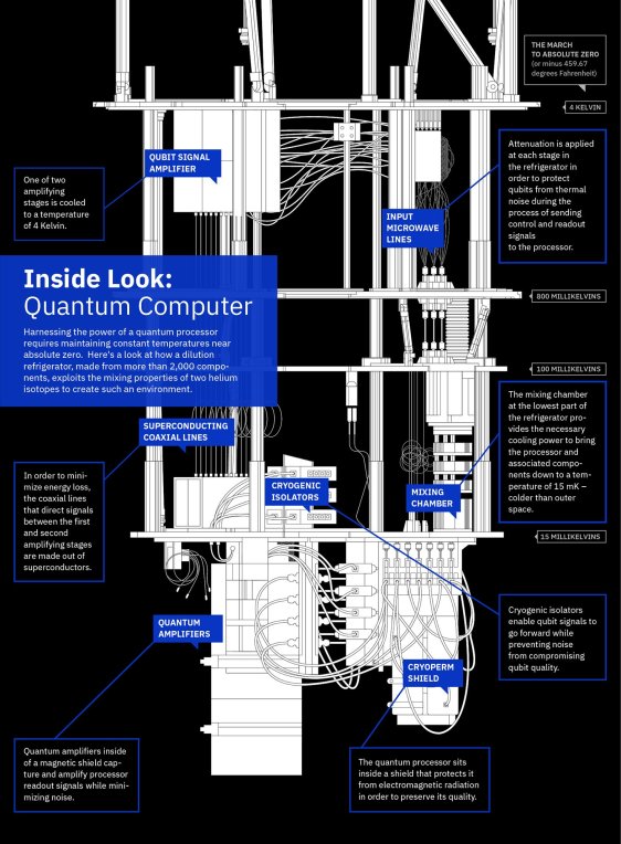
Figure 2. System Architecture of IBM-Q quantum architecture. Source: IBM Research
Signing up to use the IBM-Q pubic systems is extremely easy. Go to the qx community page and sign-up and you can get an access code. The best way to use it is with Python Jupyter so download the most recent Anaconda distribution.
The IBM-Q qiskit software stack is how we program the system. Ali Javadi-Abhari and Jay M. Gambetta have an excellent series of articles on Medium describing it. The current state of the art in the hardware is what they call “noisy intermediate-scale quantum computers (NISQ)”. The software stack is designed to allow researchers to explore several levels of NISQ computing. There are for components.
- Qiskit Terra. This is the core software platform containing all the Python APIs for describing quantum circuits and the interface to submit them to the hardware and simulators. There are many qubit operators in Tera. See this notebook for a good sample.
- Qiskit Aqua. This is the high-level application layer. It contains templates for building advanced applications in areas including chemistry, optimization and AI. (We will discuss this in more depth in part 2 of this article.)
- Qiskit Aer. Qiskit has several different simulators that run in the cloud or locally on your laptop.
The unitary_simulator. The standard operations on a quantum circuit are all unitary operations. The unitary_simulator computes the result of computation and displays the result as a complex unitary matrix.
The statevector_simulator allows you to initialize a mullti-qubit to an arbitray unit combination of the basis vectors and it will do the simulation in terms of the state vectors.
The qasm_simulator provides a detailed device level simulator that takes into account the fact that the hardware is noisy. We will illustrate this simulator below
A Quantum “Hello World” example.
Qiskit is a programming system based on compiling Python down to the basic assembly language of the IBM-Q hardware (or to the format needed by one of the simulators). For a simple “hello world” example we will use the simple demonstration of entanglement describe in the mathematical introduction section above. We start with two qubits in |0> state and apply the H transform to the first and then the controlled not (Cnot) operation to the pair. We next measure the first qubit and then the second. If they have become properly entangle then if the first was measured at a 1 then the second will be a 1. If the first is a 0, then the second will be measured as a zero.
This code is based on the sample by Jay Gambetta and Ismael Faro. Using Jupyter we start by loading the libraries we will use and then load our account information (this was established earlier on the local machine earlier using the IBMQ.save_account(‘…. Key …’) operation. With the account information we can inquire about the backend quantum systems we are allowed to use. There are three: two are hardware and one is the cloud-based qasm-simulator.
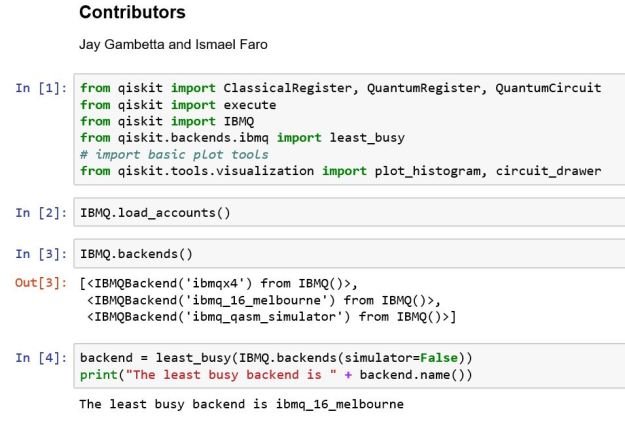
In line [4] we ask for the least busy of machines and it is the 16 qubit system.
The next step is to define the program. We declare an array of 2 qubit registers and 2 classical 1- bit registers. As shown below, we create a circuit consisting these two resources. We apply the H operator to the first qubit and the Cnot to the first and the second. Finally, we measure both.

We have not executed the circuit yet, but we can draw it. There is a standard way quantum circuits are drawn which is similar to a musical score. The registers (both quantum and classical) are drawn has horizontal lines and operators are placed on the lines in temporal order from left to right.
As you can see, the H gate is simply represented as a box. The controlled not consists of a dot on the “control” qubit and a circle on the “controlled” instance. Recall that the value of the control determines what happens to the second qubit. Of course, we can’t know the result until we do the measurement and that is represented with a little dial and a line to the output classical bit.
We next execute our circuit on the ibmq_16_melbourne hardware. We will run it 1000 times so we can get some interesting statistics.
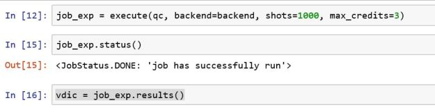
The execute command is a type of “future” call. It returns a placeholder for the result. The actual job will go into a queue and we can monitor the status. When complete we can get the data. The data is always returned from the experiment as a Python dictionary with keys labeled 0x0 for the basis |00>, ox1 for the basis vector |01> and 0x2 for |10> and 0x3 for |11>.
As we can see from the results below, the hardware is indeed noisy. The two bits are corelated 92.1% of the time. We can also plot a histogram to see the results.
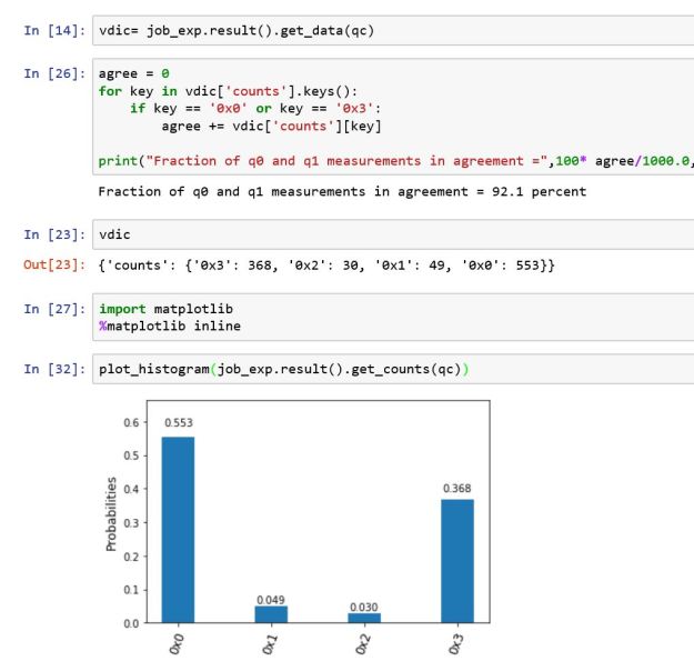
Given that we should have created the Bell state 1/√2(|00> + |11>) with our two qubit operations there should be no |01> or |10> components. But the systems are noisy, and the measurements of qubits produce results that defined by probability distributions, the outcome should not surprise us. Even the initial state of the qubit may be |0> with only 99.9% accuracy. That means it is occasionally |1>.
The IBM-Q qasm_simulator can provide a model of the execution at the device level. To use it we extract data about the device we are going to simulate. We can get very low-level details about the device and measured noise characteristics. We can also get the coupling_map that tells us how the individual qubit cells are connected on the chip.

Using this device data we can invoke the simulator. As can be seen below, we get results that are very similar to the actual experiment.


If we had used one of the other simulators we would see only the theoretically perfect results.
Microsoft Q# Quantum Programming Toolkit
Perhaps the greatest challenge when building a quantum computer is designing it so that it is stable in the presence of noise. Qubits that are too fragile will experience decoherence if they are subject to prolonged episodes of noise while they are undergoing the transformations required by a quantum algorithm. The depth of a quantum algorithm is the count of the longest path of operations in the circuit. Based on the intrinsic error characteristics of the devices and the noise there may be a limit of a few tens of thousands in the circuit dept before decoherence is likely. For some algorithms, such as those involving iteration, this limit may make it unusable. One way to solve this is by introducing error correction through massive redundancy.
Microsoft has been taking a different approach to building a qubit, one that, if successful, will yield a much more robust system without as much need for error correction. Called a topological qubit, it Is based on different physics.
Topology is the branch of mathematics that is concerned with the properties of objects that are not changed when they are perturbed or distorted. For example a torus is a 2-dimenional object that cannot be deformed into a sphere without ripping the surface of the torus. But the torus can be deformed into various other shapes, such as the surface of a coffee mug with no such tearing. Or consider points on a 1-D line as beads on a string. We cannot change their order unless we can move them from the one dimensional line to a second dimension and back to the line.  This braded structure is a topological constraints that is a global property and therefor very robust. If you can make a qubit from this property it would impervious to minor noise.
In condensed matter physics the 2016 Nobel prize was awarded to David Thouless, Duncan Haldane and Michael Kosterlitz for their work understanding strange behavior of matter when restricted to thin films. Their discovery demonstrated that the behavior had to do with the topology of 2-D surfaces. A similar discovery had to do with chains of atoms on a thin (1-D) , superconducting wire. The properties of the pair of objects at the ends of the chain were tied to the whole of the chain and not subject to minor local perturbations. Microsoft uses a similar idea to construct their “topological qubits” made from spitting electrons to form “Majorana fermion quasi-particles”. Situated at the opposite end of topological insulators they are highly noise resistant. This implies that one does not need massive redundancy in the number of qubits required for error correction that is needed for many other qubit models.
Of course the above description does not tell us much about the exact nature of their process, but several interesting theory papers exist.
The Q# programming environment.
The first iteration of a quantum computing software platform from Microsoft was based on the F# functional programming language in 2014 and called LIQUi|> (see Wecker and Svore). The current version is based on C# and is nicely embedded in Visual Studio and Visual Studio Code. You can download it here for Windows 10, Mac and Linux. The installation straightforward. There is also a Python binding but we will look at the Visual Studio version here.
The Q# programming language is designed as a hybrid between quantum operations on qubits and classical procedural programming designed to operate on a digital computer that contains the quantum device as a co-processor. Q# extends C# by introducing a number of new standard types including Qubit, Result (the result of a qubit measurement), unit (indicating an operator returns no result) and several additional operators. A complete description of the operational semantics is defined on the Q# link above. For our purposes here any Java or C# program should be able to follow the code.
There are two standard libraries and a set of research libraries. The standard libraries include
- Prelude: the collection of logic, libraries and runtime specific to a particular quantum computer architecture.
- Cannon: The hardware independent library of primitive operator that can be used as part of quantum algorithm design.
There is also a set of excellent standard libraries that include important topics like amplitude magnification, quantum Fourier Transforms, iterative phase estimation and other topics more advanced than this article can cover. There is also a set of research libraries with a focus on applications in Chemistry and Quantum Chemistry.
Hello World in Microsoft’s Q#
We begin by creating a new C# project with the “file->new->project” menu. If Q# has been correctly installed, you can select “Q# application” from the list of C# configurations and fill in the name for the project. In our case we are using “BellTest” and the system now shows the following.

This is almost exactly what you will find in the introduction when you download the kit. The file called operations.qs contains the main part of our algorithm. We will have two operations, one for initializing a quantum variable and one for the bulk of our algorithm.
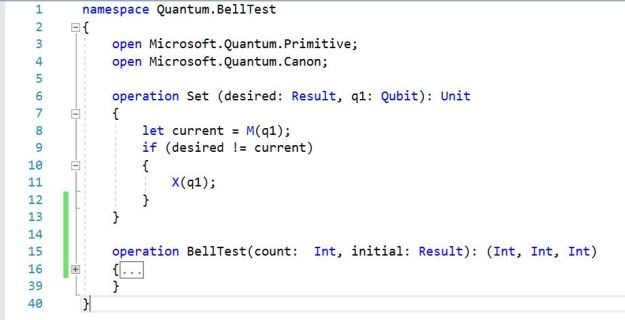
The operation Set takes a qubit and a desired value (0 or 1) and sets the qubit to have that value. It does this as follows. First we measure the qubit. Recall that measurement (in the standard basis) returns a 0 or a 1 and (in the standard basis) projects the qubit to either |0> or |1>. If measures 0 and a |1> is desired, we use the Not gate (X) to flip it. If a 1 is measured and 1 is desired no change is made, etc.
The operation BellTest takes an iteration count and an initial value we will use for qubit 1. The code is essentially identical to the example we described for qiskit. We start with an array of 2 qubits. We set qubit 0 to |0> and qubit 1 to |initial> . Next we apply H to qubit 0 and Cnot to the pair as before. We measure qubit 0 and compare it to the measurement of qubit 1. If they agree we increment a counter. If the measurement is 1 we also count that. This process is repeated count time and returns our counter values.

The main program calls BellTest two different ways: once with the initial value for qubit 1 to be 0 and one with the value of qubit 1 to be 1. In the case that both qubits are initialized to 0 we saw from the mathematical introduction that the state after the Cnot should be the Bell state 1/√2(|00> + |11>). Consequently, after the measurements both qubits should always agree: if one is 0 the other is 0 and if one is 1 the other is 1. However if qubit 1 is initialized to 1 the situation is different. Evaluating the state mathematically we get

Hence, we should see that the two qubits never agree when measured. The main program that drives this experiment is
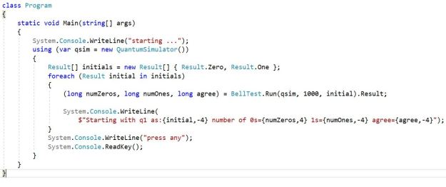
which runs BellTest 1000 times with each configuration of qubit 1. The results are below.

These results agree with the theoretical result. The only probabilistic effect is the count in the number of zeros/ones measured. Unlike the Qasm_simulator, there was no noise introduced into the initialization because the Q# simulator was not modeling a specific hardware configuration.
Conclusion
The near-term future of quantum computers will be as co-processors tightly integrated as cloud services. While IBM is now ready to start selling there systems into private clouds, others like Google and Microsoft will probably stay with a cloud service offering.
This short paper was intended to illustrate two approaches to programming quantum computers. It is certainly not sufficient to begin any serious quantum algorithm development. Fortunately, there is a ton of great tutorial material out there.
There is a great deal of exciting research that remains to be done. Here are a few topics.
- Quantum Compiler Optimzation. Given the problem of qubit decoherence over time, it is essential that quantum algorithms terminate in as few step as possible. This is classic compiler optimization.
- Efficient error correction. If you have a great quantum algorithm that can solve an important problem with 100 qubits, but the error correction requires 1000 qubits, the algorithm may not be runnable on near term machines.
- Breakthrough algorithmic demonstrations. “Quantum supremacy” refers to concrete demonstrations of significant problem solutions on a quantum computer that cannot be duplicated on a classical machine. In some cases this is argued to be algorithms that are “exponentially” faster than the best classical algorithm. However, good quantum algorithms may lead to the discovery of classical algorithms that are quantum inspired. For example, here is one for recommendation systems.
Part 2 of this report will address the application of quantum computing to AI and machine learning. This is both a controversial and fascinating topic.
