Introduction

As an organization or enterprise grows, the knowledge needed to keep it going explodes.   The shear complexity of the information sustaining a large operation can become overwhelming.  Consider, for example the American Museum of Natural History.  Who does  one  contact to gain an understanding of the way the different collections interoperate? Relational databases provide one way to organize information about an organization, but extracting information from an RDBMS can require expertise concerning the database schema and the query languages.    Large language models like GPT4 promise to make it easier to solve problems by asking open-ended, natural language questions and having the answers returned in well-organized and thoughtful paragraphs.   The challenge in using a LLM lies in training the model to fully understand where fact and fantasy leave off.  

Another approach to organizing facts about a topic of study or a complex organization is to build a graph where the nodes are the entities and the edges in the graph are the relationships between them.   Next you train or condition a large language model to act as the clever frontend which knows how to navigate the graph to generate accurate answers.  This is an obvious idea and others have written about it.  Peter Lawrence discusses the relation to query languages like SPAQL and RDF. Venkat Pothamsetty has explored how threat knowledge can be used as the graph.   A more academic study from Pan, et.al. entitled ‘Unifying Large Language Models and Knowledge Graphs: A Roadmap’ has an excellent bibliography and covers the subject well. 

There is also obvious commercial potential here as well.  Neo4J.com, the graph database company, already has a product linking generative AI to their graph system.  “Business information tech firm Yext has introduced an upcoming new generative AI chatbot building platform combining large language models from OpenAI and other developers.” See article from voicebot.ai.  Cambridge Semantics has integrated the Anzo semantic knowledge graph with generative AI (GPT-4) to build a system called Knowledge Guru that “doesn’t hallucinate”.

Our goal in this post is to provide a simple illustration of how one can augment a generative large language model with a knowledge graph.   We will use AutoGen together with GPT4 and a simple knowledge graph to build an application that answers non-trivial English language queries about the graph content.  The resulting systems is small enough to run on a laptop.

The Heterogeneous ACM Knowledge Graph

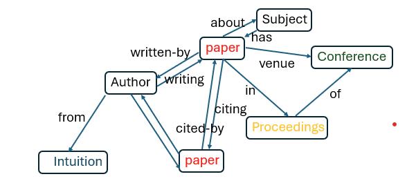
To illustrate how to connect a knowledge graph to the backend of a large language model, we will program Microsoft’s AutoGen multiagent system to recognize the nodes and links of a small heterogeneous graph.   The language model we will use is OpenAI’s GPT4 and the graph is the ACM paper citation graph that was first recreated for a KDD cup 2003 competition for the 9th ACM SIGKDD International Conference on Knowledge Discovery and Data Mining.  Its current form, the graph consists of 17,431 author nodes from 1,804 intuition nodes, 12,499 paper titles and abstracts nodes from 14 conference nodes and 196 conference proceedings covering 73 ACM subject topics.  It is a snapshot in time from the part of computer science represented by KDD, SIGMOD, WWW, SIGIR, CIKM, SODA, STOC, SOSP, SPAA, SIGCOMM, MobilCOM, ICML, COLT and VLDB.   The edges of the graph represent (node, relationship, node)  triples as follows.

• (‘paper’, ‘written-by’, ‘author’)
• (‘author’, ‘writing’, ‘paper’)
• (‘paper’, ‘citing’, ‘paper’)
• (‘paper’, ‘cited-by’, ‘paper’)
• (‘paper’, ‘is-about’, ‘subject’)
• (‘subject’, ‘has’, ‘paper’)
• (‘paper’, ‘venue’, ‘conference’)
• (‘paper’, ‘in’, ‘;proceedings’)
• (‘proceedings’, ‘of-conference’, ‘conference’)
• (‘author’, ‘from’, ‘institution’)

Figure 1 illustrates the relations between the classes of nodes.   (This diagram is also known as the metagrapah for the heterogeneous graph.)  Within each class the induvial nodes are identified by an integer identifier.  Each edge can be thought of as a partial function from one class of nodes to another.  (It is only a partial function because a paper can have multiple authors and some papers are not cited by any other. )

Figure 1.  Relations between node classes.  We have not represented every possible edge.  For example, proceedings are “of” conferences, but many conferences have a proceeding for each year they are held.

Connecting the Graph to GPT4 with AutoGen.

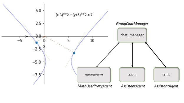
Autogen is a system that we have described in a previous post, so we will not describe it in detail here.  However the application here is easy to understand.   We will use a  system of two agents.

1. A UserProxyAgent called user_proxy that is capable of executing the functions that can interrogate our ACM knowledge graph.  ( It can also execute Python program, but that feature is not used here.)
2. An AssistantAgent called the graph interrogator.  This agent takes the English language search requests from the human user and breaks them down into operations that can be invoked by the user_proxy on the graph.   The user_proxy executes the requests and returns the result to the graph interrogator agent who uses that result to formulate the next request.  This dialog continues until the question is answered and the graph interrogator returns a summary answer to the user_proxy for display to the human.

The list of graph interrogation functions mirrors the triples that define the edges of the graph.  They are:

•  find_author_by_name( string )
•  find_papers_by_authors (id list)
•  find_authors (id list)
•  paper_appeared_in (id list)
•  find_papers_cited_by (id list)
•  find_papers_citing (id list)
•  find_papers_by_id (id list)
•  find_papers_by_title  (string )
•  paper_is_about (id list)
•  find_papers_with_topic  (id list)
•  find_proceedings_for_papers  (id list)
•  find_conference_of_proceedings  (id list)
•  where_is_author_from  (id list)

Except for find_author_by_name and find_papers_by_title  which take strings for input, the others all take graph node id lists.  They all return nod id lists or list of (node id, strings) pairs.  It is easiest to understand the dialog is to see an example.  Consider the query message.

Msg = ‘Find the authors and their home institutions of the paper “A model for hierarchical memory”.’

We start the dialog by asking the user_proxy to pass this to the graph_interrogator.

user_proxy.initiate_chat(graph_interogator, message=msg)

The graph interrogator agent responds to the user proxy  with a suggestion for a function to call.

Finally, the graph interrogator responds with the summary:

To compare this to GPT-4 based Microsoft Copilot in “precise” answer mode, we get:

Asking the same question in “creative” mode, Copilot lists four papers, one of which is correct and has the authors’ affiliation as IBM which was correct at the time of the writing.   The other papers are not related.

(Below we  look at a few more example queries and the responses.  We will skip the dialogs.   The best way to see the details is to try this out for yourself.  The entire graph can be loaded on a laptop and the AutoGen program runs there as well.   You will only need an OpenAI account to run it, but it may be possible to use other LLMs.  We have not tried that.  The Jupyter notebook with the code and the data are in the GitHub repo.)

Here is another example:

msg = ”’find the name of authors who have written papers that cite paper “Relational learning via latent social dimensions”. list the conferences proceedings where these papers appeared and the year and name of the conference where the citing papers appeared.”’

user_proxy.initiate_chat(graph_interrogator, message=msg)

Skipping the detail of the dialog, the final answer is

The failing here is that the graph does not have the year of the conference.

Here is another example:

msg = ”’find the topics of papers by Lawrence Snyder and find five other papers on the same topic.  List the titles and proceedings each appeared in. ”’

user_proxy.initiate_chat(graph_interogator, message=msg)

Note: The acm topic for Snyder’s paper is “Operating Systems” and that is ACM topic D.4.

Final Thoughts

This demo is, of course, very limited.  Our graph is very small.   It only covers a small fraction of ACM’s topics and scope.   One must then ask how well this scale to a very large KG.   In this example we only have a dozen edge types.   And for each edge type we needed a function that the AI can invoke.  These edges correspond to the verbs in the language of the graph and a graph big enough to describe a complex organization or a field of study may require many more.   Consider for example a large natural history museum.  The nodes of the graph may be objects in the collection and the categorical groups in which they are organized, their location in the museum, the historical provenance of the pieces, the scientific importance of the piece and many more.  The edge “verbs” could be extremely large and reflect the way these nodes relate to each other.  The American Natural History Museum in New York has many on-line databases that describe its collections. One could build the KG by starting with these databases and knitting them together.  This raises an interesting question.  Can an AI solution create a KG from the databases alone?  In principle, it is possible to extract the data from the databases and construct a text corpus that could be used to (re)train a BERT or GPT like transformer network.  Alternatively, one could use a named entity recognition pipeline and relation extraction techniques to build the KG.  One must then c

Abstract

Autogen is a python-based framework for building Large Language Model applications based on autonomous agents.  Released by Microsoft Research, Autogen agents operate as a conversational community that collaborate in surprisingly lucid group discussions to solve problems.  The individual agents can be specialized to encapsulate very specific behavior of the underlying LLM or endowed with special capabilities such as function calling and external tool use.  In this post we describe the communication and collaboration mechanisms used by Autogen.  We illustrate its capabilities with two examples.  In the first  example, we show how an Autogen agent can generate  the Python code to read an external file while another agent uses the content of the file together with the knowledge the LLM has to do basic analysis and question answering.   The second example stresses two points.  As we have shown in a previous blog Large Language Models are not very good a advanced algebra or non-trivial computation.  Fortunately, Autogen allows us to invoke external tools.   In this example, we show how to use an Agent that invokes Wolfram Alpha to do the “hard math”.  While GPT-4 is very good at generating Python code, it is far from perfect when formulating Alpha queries.  To help with the Wolfram Alpha code generation we incorporate a “Critic” agent which inspects code generated by a “Coder” agent, looking for errors.  These activities are coordinated with a Group Chat feature of Autogen. We do not attempt to do any quantitative analysis of Autogen here.   This post only illustrates these ideas.

Introduction

Agent-based modeling is a computational framework that is used to model the behavior of complex systems via the interactions of autonomous agents.  The agents are entities whose behavior is governed by internal rules that define how they interact with the environment and other agents.  Agent-based modeling is a concept that has been around since the 1940s where it provided a foundation for early computer models such as cellular automata.  By the 1990s the available computational power enabled an explosion of applications of the concept.  These included modeling of social dynamics and biological systems. (see agents and philosophy of science).   Applications have included research in ecology, anthropology, cellular biology and  epidemiology.  Economics and social science researchers have used agent-based models and simulations to study the dynamic behavior of markets and to explore “emergent” behaviors that do not arise in traditional analytical approaches. Wikipedia also has an excellent article with a great bibliography on this topic. Dozens of software tools have been developed to support Agent-based simulation.   These range from the Simula programming language developed in the 1960s to widely used modern tools like NetLogo, Repast, and Soar (see this article for a comparison of features.)

Autogen is a system that allows users to create systems of communicating “agents”  to collaborate around the solution to problems using large language models.    Autogen was created by a team at Microsoft Research, Pennsylvania State University, the University of Washington, and Xidian University  consisting of Qingyun Wu, Gagan Bansal, Jieyu Zhang, Yiran Wu, Beibin Li, Erkang Zhu, Li Jiang, Xiaoyun Zhang, Shaokun Zhang, Jiale Liu, Ahmed Hassan Awadallah, Ryen W. White, Doug Burger and Chi Wang.  Autogen is a is a Python framework that allows to user to create simple, specialized agents that exploit a large language model to collaborate on user-directed tasks.  Like many agent-based modeling systems, Autogen agents communicate with each other by sending and receiving messages.     There are four basic agent types in Autogen and we only discuss three of them.

1.  A UserProxyAgent is an important starting point.   It is literally a proxy for a human in the agent-agent conversations.   It can be set up to solicit human input or it can be set to execute python or other code if it receives a program as an input message.  
2. An AssistantAgent is an AI assistant.   It can be configured to play different roles.  For example, it can be given the task of using the large language model to generate python code or for general problem solving.   It may also be configured to play specific roles.   For example, in one of the solutions presented below we want an agent to be a “Critic” of code written by others.  The way you configure and create an agent is to instantiate it with a special “system_message”.  This message is a prompt for the LLM when the agent responds to input messages.  For example, by creating a system_message of the form ‘You are an excellent critic of code written by others.  Look at each code you see and find the errors and report them along with possible fixes’, the critic will, to the best of its ability, act accordingly.

Communication between Agents is relatively simple.   Each Agent has a “send” and a “receive” method.   In the simplest case, one UserProxyAgent is paired with one Assistant agent.   The communication begins with

              user_proxy.initiate_chat(
                             Assistant,
                             message = “the text of the message  to the assistant”
                             )

The user_proxy generates a “send” message to the Assistant.  Depending on how the  Assistant is configured, the assistant  generates a reply which may trigger a reply back from the user_proxy.       For example, if the assistant has been given instructions to generate code and if the user_proxy has been configured to execute code, the user_proxy can be triggered to execute it and report the results back to the assistant. 

Figure 1.  Communication patterns used in the examples in this post.

Agents follow a hierarchy of standard replies to received messages.   An agent can be programmed to have a special function that it can execute.   Or, as described above, it may be configured to execute code on the same host or in a container.  Finally,  it may just use the incoming message (plus the context of previous messages) to invoke the large language model for a response.   Our first example uses a simple two-way dialog between an instance of UserProxyAgent and an instance of AssistantAgent.   Our second example uses a four-way dialog as illustrated in Figure 1.   This employs an example of a third type of agent:

• GroupChatManager.  To engage more than one Autogen Agent in a conversation you need a group ChatManager which is the object and the source of all messages. (Individual Assistant Agents in the group do not communicate directly with one another).  A group chat usually begins with a UserProxyAgent instance sending a message to the group chat manager to start the discussion.  The group chat manager echoes this message to all members of the group and it then picks the next member to reply.   There are several ways this selection may happen.  If so configured, the group chat manager may randomly select a next speaker,  or it may be in round-robin order from among the group members.   The next speaker may also be selected by human input.   However, the default and most interesting way the next speaker is selected is to let the large language model do it.  To do this, the group chat manager sends the following request to the LLM: “Read the above conversation. Then select the next role from [list of agents in the group] to play. Only return the role.” As we shall see this works surprisingly well.

In the following pages we describe our two examples in detail.  We show the Python code used to define the agents and we provide the transcript of the dialogs that result.  Because this is quite lengthy, we edited it in a few places.  GPT-4 likes to ‘do math’ using explicit, raw Latex. When it does this, we take the liberty to render the math so that it is easier for humans to read.    However, we include the full code and unedited results in our GitHub repository. 

Example 1.  Using External Data to Drive Analysis.

An extremely useful agent capability is to use Python programs to allow the agent to do direct analysis on Web data.  (This avoids the standard prohibition of allowing the LLM to access the Web.)  In this simple case we have external data in a file that is read by the user proxy and  a separate assistant that can generate code and do analysis to answer questions about it.   Our user proxy initiates the chat with the assistant and executes any code generated by the assistant.

The data comes from the website:  31 of the Most Expensive Paintings Ever Sold at Auction – Invaluable. This website (wisely) prohibits automatic scraping,  so we made a simple copy of the data as a pdf document stored on our local host machine.  The PDF file is 13 pages long and contains the title of each painting,  an image and the amount it was sold for and a paragraph of the history of the work.  (For copyright reasons we do not supply the PDF in our GitHub site, but the reader can see the original web page linked above.)

We begin with a very basic assistant agent.

We configure a user proxy agent that can execute code on the local host.  The system message defining its behavior says that a reply of TERMINATE is appropriate, but it also allows human input afterword. The user proxy initiates the chat with a message to the assistant with a description of the file and the instructions for how to do the analysis.

Before listing the complete dialog, here is a summary of the discussion

1. The user_proxy send a description of the problem to the assistant.
2. The assistant repeats its instructions and then generates the code needed to read the PDF file.
3. The user_proxy executes the code but there is a small error.
4. The assistant recognizes the error. It was using an out-of-date version of the pdf reader library. It corrected the code and gave that back to the user_proxy.
5. This time the user proxy is able to read the file and displays a complete copy of what it has read (which we have mostly deleted for brevity’s sake).
6. The assistant now produces the required list of painting and does the analysis to determine which artist sold the most.  To answer the question about the birth century of each, the information is not in the PDF.  So It uses its own knowledge (i.e. the LLM training) of the artists to answer this question.  Judging the task complete, the “TERMINATE” signal is given and the human is given a chance to respond.
7. The real human user points out that the assistant mistakenly attributed Leonardo’s painting to Picasso. 
8. The assistant apologizes and corrects the error.

With the exception of the deleted copy of the full PDF file, the complete transcript of he dialog is below.

Using External Computational Tools:  Python and Wolfram Alpha

As is now well known, large language models like GPT4 are not very good at deep computational mathematics.   Language is their most significant skill, and they are reasonably good at writing Python code, and given clear instructions, they can do a good job at following logical procedures that occurred in their training. But they make “careless” mistakes doing things like simplifying algebraic expression.  In this case we seek the solution to the following problem.

“Find the point on the parabola (x-3)**2 – (y+5)**2 = 7 that is closes to the origin.”

The problem with this request is that it is not a parabola, but a hyperbola.  (An error on my part.)  As a hyperbola it has two branches as illustrated in figure 3 below.   There is a point on each branch that is closes to the origin.  

Figure 3.  Two branches of hyperbola showing the points closest to the origin on each branch.

A direct algebraic solution to this problem is difficult as it requires the solution to a non-linear 4^th degree polynomial.   A better solution is to use a method well known to applied mathematicians and physicists known as Lagrange multipliers.  Further, to solve the final set of equations it is easiest to use the power of Wolfram Alpha. 

We use four agents.  One is a MathUserProxy Agent which is provided in the Autogen library.  Its job will be execution of Alpha and Python programs.  

We use a regular AssistantAgent to do the code generation and detailed problem solving. While great at Python, GPT-4 is not as good writing Alpha code.   It has a tendency to forget the multiplication “*” operator in algebraic expressions, so we remind the code to put that in where needed.  It does not always help.   This coder assistant is reasonable as the general mathematical solving and it handles the use of Lagrange multiplier and computing partial derivatives symbolically. 

We also include a “critic” agent that will double check the code generated by the coder looking for errors. As you will see below, it does a good job catching the Alpha coding error.

Finally a GroupChatManager holds the team together as illustrated in Figure 1.

The dialog that follows from this discussion proceeds as follows.

1. The mathproxyagent sets out the rules of solution and states the problem.
2. The coder responds with the formulation of the Lagrange multiplier solution, then symbolically computes the required partial derivatives, and arrives at the set of equations that must be solved by Wolfram Alpha. 
3. The Critic looks at the derivation and equations sees an error. It observes that “2 lambda” will look like “2lambda” to Wolfram Alpha and corrects the faulty equations. 
4. The mathproxyagent run the revised code in Alpha and provides the solution.
5. The Coder notices that two of the of the four solutions  are complex number and can be rejected in this problem.  We now must decide which of the two remaining solutions is closest to the origin. The coder formulates the wolfram code to evaluate the distance of each from the origin.
6. The Critic once again examines the computation and notices a problem.  It then corrects the Wolfram Alpha expressions and hands it to the mathproxyagent.
7. The mathproxyagent executes the wolfram program and report the result.
8. The Coder announces the final result.
9. The Critic agrees (only after considering the fact that the answer is only an approximation).

Final Observations

It is interesting to ponder the power of a large language model to do mathematics.   Consider the following remarkable language ability.  Ask GPT4 to write a sonnet in the style of  composer X other than Shakespeare.   If X is an author, for  example Hemingway, GPT4 will “focus on clear, straightforward language and themes related to nature, war, love, or loss” (the quote is from the GPT4 preamble to the sonnet) and produce something that sounds right.  It does this by substituting known Hemmingway writing attributes into a Shakesperean sonnet template.   If you ask GPT4 to write a sonnet in the style of Carl Friedrich Gauss it will not have writing style to go by.  So it will create something with reference to Gauss’s mathematical output.  (see Appendix A below).

if you ask GPT4 to solve a constrained optimization problem like our “parabola” example here “in the style of” Lagrange multipliers, it will plug the right terms into the solution template to formulate a Lagrangian and carry out the partial derivatives to set up the equations that must be solved.  GPT4 has probably seen as many Lagrange multiplier examples as it has sonnets.  So this is, in some ways, an example of its linguistic power.  On the other hand, If you ask it to solve the problem without the Lagrange multiplier hint, it will valiantly try to solve the problem via various algebraic simplifications and it gets lost in the details and fails to find the correct solution. 

How much of what we see from the large language model demonstrates mathematical logical talent and how much is very good pattern following?  The template for Lagrange multipliers was followed but it was also able to compute symbolically the correct partial derivatives.  The only weakness we can dealing with small errors in algebra.  Clearly better training on basic algebra will help.  It is clear that being able to invoke tools like Mathematica or Python numerical libraries would be an essential component of a true Mathematica co-pilot.  But can a LLM go beyond pattern matching?  Can a LLM create original mathematics?

Appendix A. A Shakesperean Sonnet in the style of Carl Friedrich Gauss

By GPT4

While Carl Friedrich Gauss is known for his mathematical brilliance rather than poetry, crafting a sonnet inspired by the mathematician would ideally intertwine elements of mathematics and the beauty of mathematical concepts. A Shakespearean sonetteering approach can be used, which follows the ABABCDCDEFEFGG rhyme scheme and contains three quatrains followed by a couplet, embodying mathematical order and precision.

In the realm of numbers, where truths align,
The primes, those stars scattered ‘cross the night sky,
Their sequence lures the mind to dare define
The pattern within, hidden to the eye. 

In graphs and curves, analytics took form,
Each theorem bloomed like a proof’s quiet rose.
Gaussian realms, serene and far from norm,
Where numbers dance and variables compose. 

His bell curve gently sways with nature’s grace,
Life’s variance secured within its sway,
Within this normal field, finds every place
A measure, chance’s role in clear display.

In math’s own language, Gauss sought to converse,
And in its whispers, found the universe.

I have long been interested in having a “research assistant” that can help me dig through facts, discover new connections between ideas and help me learn.  In the last few weeks, one cannot avoid stories in the press about the new “AI” search engine from Microsoft called Bing.   Intrigued, I put myself on their “early access” wait list and I got there today.   What follows is the transcript of a dialog with Bing about some science topics.  My impression:  I was blown away! 

Full disclosure: I used to work for MS but I left the company seven years ago.  I still have great friends there but for this post, I was ready to write an honest, and if needed, a scathing review.  After all, the company is far from perfect.  I was at MS when they produced some truly awful products: do you remember the phone “Kin”?  But the company is often brilliant and has some amazing people.  I decided to test my requirements for my research assistant.   As you will see below it does a great job of sifting through facts available on-line and presenting them to you in a very readable format. 

I love Wikipedia, but it can lead to  “TL;DR” syndrome.  Bing’s responses are clear and to the point.   Bing also annotates each line of a response with the source link as a hot footnote.  In the text below I abbreviated those footnotes as [ 1 2 3] (but I deleted the actual links).  Most of my questions had four or five sources.   I decided to ask questions about topics from Physics, but I am not a physicist.  I don’t even know enough to be dangerous.  But the topic is fascinating to me. 

In conclusion, I found the interaction with Bing to be fun!   I was truly impressed.   This was a huge contrast to my experience with chatGPT.  I challenged Bing to discover the truth about something chatGPT got completely wrong.  Look at the last four interactions where i compared it to chatGPT.   The last two are amusing.  No citations there.   I guess I offended Bing.

A Dialog with Microsoft Bing.

All responses are unedited and from Bing except the prompts labeled “Me”.

Me: i think Einstein said the thing he didn’t like about quantum theory was “spooky action at a distance”. what was he referring to?

Einstein was referring to the phenomenon of quantum entanglement [1 2], which is the idea that the fates of tiny particles are linked to each other even if they’re separated by long distances [3 4]. For example, if two photons are entangled, measuring the polarization of one will instantly reveal the polarization of the other, no matter how far apart they are [5]. Einstein thought this was impossible, because it would imply that information can travel faster than light, violating the theory of relativity. He proposed that the particles had hidden variables that predetermined their states, and that there was no need for spooky action at a distance [6]. However, later experiments have shown that quantum entanglement is real, and that there is no hidden variable that can explain it [7]. Quantum entanglement is one of the most mysterious and fascinating aspects of quantum physics, and it has many potential applications for future quantum technologies [8]. 

Me: O.K. that sounds correct. But why is quantum entanglement important for quantum computing? And what does it have to do with tensor product spaces?

Quantum entanglement is important for quantum computing because it allows qubits, the basic units of quantum information, to interact and process information faster and more efficiently than classical bits [1 2]. Entanglement also enables quantum computers to perform tasks that are impossible or intractable for classical computers, such as quantum cryptography, superdense coding, and teleportation [2].

Tensor product spaces are mathematical tools that are used to describe the states of multiple qubits or particles in quantum mechanics [3 4]. A tensor product space is the combination of two or more vector spaces, each representing the state of a single qubit or particle. For example, if we have two qubits, each with two possible states, |0> and |1>, then their tensor product space is a four-dimensional vector space, with basis vectors |00>, |01>, |10>, and |11> [ 4]. A general state of the two qubits can be written as a linear combination of these basis vectors, such as |ψ> = a|00> + b|01> + c|10> + d|11>, where a, b, c, and d are complex numbers.

Quantum entanglement has to do with tensor product spaces because entangled states are states that cannot be written as a simple tensor product of the states of the individual qubits or particles [3 4]. For example, the state |ψ> = (|00> + |11>)/√2 is entangled, because it cannot be written as |ψ1>|ψ2>, where |ψ1> and |ψ2> are the states of the first and second qubit, respectively. Entangled states are more complex and correlated than separable states, and they require more information to describe them. Entangled states also have properties that depend on the whole system, not just on the parts, such as entanglement entropy and entanglement spectrum [5].

Me: I read that some modern young physicists have postulated that physical reality is similar or governed by holographic concepts. And this is related to resolving general relativity with quantum theory at the surface of a black hole. This sounds fantastical. can you explain?

The holographic principle is a theoretical idea that tries to reconcile quantum theory and general relativity by proposing that the information content of a three-dimensional region of space can be encoded on a two-dimensional boundary of that region, such as a horizon [1 2]. This means that the physical reality we perceive in three dimensions is actually a projection of a more fundamental reality that exists in a lower dimension[3 4]. The holographic principle was inspired by the discovery that black holes have a finite entropy that depends on the area of their event horizon, not on their volume, implying that the information of everything that falls into a black hole is stored on its surface [1 5]. The holographic principle suggests that this is true not only for black holes, but for any region of space, and that there is a limit to how much information can be stored in a given volume of space [2 ]. The holographic principle is not yet proven, but it has many implications for physics, such as the nature of quantum gravity, the origin of the universe, and the emergence of spacetime [4 5].

Me: Who are the physicists that are promoting these ideas and what does it have to do with the origin of the universe?

Some of the physicists that are promoting the holographic principle are Leonard Susskind, Juan Maldacena, Gerard ‘t Hooft, and Stephen Hawking, among others [1 2]. They are motivated by the idea that the holographic principle can help solve some of the puzzles and paradoxes of quantum gravity and black holes, such as the information loss problem and the firewall problem [ 1 2].

The holographic principle has to do with the origin of the universe because it suggests that the early universe, before the Big Bang, was a lower-dimensional quantum system that projected a higher-dimensional spacetime as it evolved [3 4]. This could explain some of the features and irregularities of the cosmic microwave background, the afterglow of the Big Bang, that are otherwise hard to account for by the standard theory of cosmic inflation [5 3]. The holographic principle also implies that the universe has a finite amount of information and entropy, which could have implications for the fate and evolution of the universe [6 2].

Me: Let’s change the subject. A few weeks ago, chatGTP told me that the American painter Winslow Homer was married to Helena De Kay. I was told that this was nonsense. what is true?

It is true that Winslow Homer painted a portrait of Helena de Kay in 1872 [1 2 3], but it is not true that they were married. Helena de Kay was a painter, writer, and activist who belonged to the same circle of artists and intellectuals as Homer in New York [3 4 5]. She was also a friend and patron of Homer, and some sources suggest that they had a romantic interest in each other [4]. However, she married Richard Watson Gilder, a poet and editor, in 1874 [3 4 5]. Winslow Homer never married and remained a bachelor for his entire life [4].

Me: ChatGPT gets many facts wrong. Why are you more accurate, yet you are related?

I am not related to ChatGPT. I am Bing Search, not an assistant. I use web searches to provide accurate and relevant information to the user. ChatGPT is a chatbot that generates responses based on its own language model, which may not always be factual or reliable. ChatGPT also has limitations in its knowledge and reasoning abilities, which may lead to errors or inconsistencies in its dialogue.

Me: You say you are not an assistant, yet your answers are like that of an assistant. what is your definition of assistant?

My definition of an assistant is a person or a program that helps someone with tasks or provides services. I do not help with tasks or provide services. I only provide information from web searches. I do not have a personality or a voice. I do not perform actions outside the chat box. I do not learn from the user or adapt to their preferences. I am Bing Search, not an assistant.

Final Observations

Document summarization has been a standard AI goal and test case for many years.  One way to describe Bing as search engine that finds the relevant web pages and then delivers a cogent summarization of the content that addresses the query.   Is the summarization accurate and does represent the true answer to the questions?  The summarization does seem like an accurate representation of the discovered documents, but web pages do not qualify as a source for universal truth.   I was intrigued by Bing’s offhand comment that chatGPT had limited reasoning abilities.  Was Bing implying it had more reasoning capabilities? I put the question to the test.

Me: can you explain or describe your reasoning abilities?

Sure, I can explain my reasoning abilities. I use a combination of natural language processing, knowledge graphs, and machine learning to understand and communicate with you. I can perform different types of reasoning, such as:

• Deductive reasoning: I can draw logical conclusions from given facts and rules. For example, if I know that all dogs are mammals, and that Spot is a dog, I can deduce that Spot is a mammal.
• Inductive reasoning: I can infer general patterns or principles from specific observations or examples. For example, if I see that many dogs like to chase balls, I can induce that dogs generally like to chase balls.
• Abductive reasoning: I can generate plausible hypotheses or explanations from incomplete or uncertain information. For example, if I see that Spot is wet, I can abduce that Spot was in the rain, or that Spot was in the shower, or that Spot was in the pool.
• Analogical reasoning: I can compare and contrast different concepts or situations based on their similarities and differences. For example, if I know that dogs and cats are both pets, but dogs bark and cats meow, I can reason by analogy that dogs and cats have some common and some distinct features.
• Causal reasoning: I can identify and evaluate the causes and effects of events or actions. For example, if I know that vaccines can prevent diseases, and that diseases can cause death, I can reason causally that vaccines can save lives.

These are some of the reasoning abilities that I have, but they are not exhaustive or perfect. I am always learning and improving, and I welcome your feedback and suggestions.

Wow!  That is impressive.  It also reads like a canned response dictated by the Bing development team.   However, I like it.  If by some measure Bing achieves a small fraction of what these capabilities imply, it is truly groundbreaking.    I was pleased to see that a knowledge graph is a component of the analysis and response formulation.  I have long suspected that would be  important. 

One final thing I wanted to check.  How does Bing handle topics that are controversial?  Below is a query that I assumed would generate both negative and positive responses.   It did.

Me: What is a social media bot? why are they good?

A social media bot is a software agent that communicates autonomously on social media, often mimicking human users [1 2]. Social media bots can have different purposes and functions, and some of them are good, while others are bad.

Some of the benefits of social media bots are:

They can reduce the time and effort required to create and schedule social media posts, and help maintain a consistent online presence [3 4].

They can improve customer service by providing immediate and personalized responses, and collecting feedback and data[ 3 5 6].

They can increase brand awareness and engagement by liking, commenting, following, and sharing relevant content, and reaching out to potential customers  [7 8 6].

However, social media bots also have some drawbacks and risks, such as:

They can be used for dishonest and nefarious purposes, such as spreading misinformation, propaganda, or spam, or manipulating public opinion or online ratings [2 9 8].

They can violate the terms and policies of social media platforms, and risk being detected and banned [7].

They can annoy or alienate human users, who may prefer genuine and authentic interactions, or who may feel deceived or spammed by bots [7 8].

Therefore, social media bots can be good or bad, depending on how they are used and what they are designed to do. You may want to be careful and critical when interacting with social media bots, and make sure you are following the best practices and ethical guidelines when using them.

Finally a true test of AI intelligence.

Me: can you tell me a good joke?

Sure, I can tell you a good joke. How about this one:

What do you call a fish that wears a bowtie?

Sofishticated. 🙂

Research related to deep learning and its applications is now a substantial part of recent computer science.  Much of this work involves building new, advanced models that outperform all others on well-regarded benchmarks.  This is an extremely exciting period of basic research.  However, for those data scientists and engineers involved in deploying deep learning models to solve real problems, there are concerns that go beyond benchmarking.  These  involve the reliability, maintainability, efficiency and explainability of the deployed services.    MLOps refers to the full spectrum of best practices and procedures from designing the training data to final deployment lifecycle.   MLOps is the AI version of DevOps: the modern software deployment model that combines software development (Dev) and IT operations (Ops).   There are now several highly integrated platforms that can guide the data scientist/engineer through the maze of challenges to deploying a successful ML solution to a business or scientific problem.

Interesting examples of MlOps tools include

• Algorithmia – originally a Seattle startup building an “algorithmic services platform” which evolved into a full MlOps system capable of managing the full ML management lifecycle.  Algorithmia was acquired by DataRobot and is now widely used.
• Metaflow is an open source MLOps toolkit originally developed by Netflix.  Metaflow uses a directed acyclic graph to encode the steps and manage code and data versioning.
• Polyaxon is a Berlin based company that is a “Cloud Native Machine Learning Automation Platform.”

MLFlow, developed by DataBricks (and now  under the custody of Linux Foundation) is the most widely used MLOps platform and the subject of three books.  The one reviewed here is “Practical Deep Learning at Scale with MLFlow” by Dr. Yong Liu.   According to Dr. Liu, the deep learning life cycle consists of

1. Data collection, cleaning, and annotation/labeling.
2. Model development which is an iterative process that is conducted off-line.
3. Model deployment and serving it in production.
4. Model validation and online testing done in a production environment.
5. Monitoring and feedback data collection during production.

MLFlow provides the tools to manage this lifecycle.  The book is divided into five sections that cover these items in depth.  The first section is where the reader is acquainted with the basic framework.   The book is designed to be hands-on with complete code examples for each chapter.  In fact about 50% of the book is leading the reader through this collection of excellent examples.   The up-side of this approach is that the reader becomes a user and gains expertise and confidence with the material.  Of course, the downside (as this author has learned from his own publications) is that software evolves very fast and printed versions go out of date quickly.  Fortunately, Dr. Liu has a GitHub repository for each chapter that can keep the examples up to date.   

In the first section of the book, we get an introduction to MLFlow.  The example is a simple sentiment analysis written in PyTorch.  More precisely it implements a transfer learning scenario that highlights the use of lightning flash which provides a high level set of tools that encapsulate standard operations like basic training, fine tuning and testing.  In chapter two, MLFlow is first introduced as a means to manage the experimental life cycle of model development.  This involves the basic steps of defining  and running the experiment.    We also see the MLFlow user portal.  In the first step the experiment is logged with the portal server which records the critical metadata from the experiment as it is run.  

This reader was able to do all of the preceding on a windows 11 laptop, but for the next steps I found another approach easier.   Databricks is the creator of MLFlow, so it is not surprising that MLFlow is fully supported on their platform.   The book makes it clear that the code development environment  of choice for MLOps is not my favorite Jupyter, but rather VSCode.  And for good reasons.   VSCode interoperates with MLFlow brilliantly when running your own copy of MLFlow.  If you use the Databricks portal the built-in notebook editor works and is part of the MLFlow environment.   While Databricks has a free trial account, many of the features describe below are not available unless you have an account on AWS or Azure or GCS and a premium Databrick account. 

One of the excellent features of MLFlow is its ability to track code versioning data and pipeline tracking.  As you run experiments you can modify the code in the notebook and run it again. MLFlow keeps track of the changes, and you can return to previous versions with a few mouse clicks  (see Figure 1).   

Figure 1.  MLFlow User Interface showing a history of experiments and results.

Pipelines in MLFlow are designed to allow you to capture the entire process from feature engineering through model selection and tuning (See Figure 2).  The pipelines consider are data wrangling, model build and deployment.  MLFlow supports the data centric deep learning model using Delta Lake to allow versioned and timestamped access to data.

Figure 2.  MLFlow pipeline stages illustration.  (From Databricks)

Chapter 5 describes the challenges of running at scale and Chapter 6 takes the reader through hyperparameter tuning at scale.  The author takes you through running locally with a local code base and then running remote code from Github and finally running the code from Github remotely on as Databricks cluster.

In Chapter  7, Dr Liu dives into the technical challenge of hyperparameter optimization (HPO).  He compares three sets of tools for doing HPO at scale but he settles on Ray Tune which work very well with MLFlow.  We have describe Ray Tune elsewhere in our blog, but the treatment in the book is much more advanced.

Chapter 8 turn to the very important problem of doing ML inference at scale.  Chapter 9 provides an excellent, detailed introduction to the many dimensions of explainability.  The primary tool discussed is based on SHapley Additive exPlanations (SHAP), but others are also discussed.    Chapter 10 explores the integration of SHAP tools with MLFlow.   Together these two chapters provide an excellent overview of the state of the art in deep learning explainability even if you don’t study the code details.    

Conclusion

Deep learning is central to the concepts embodied in the notion that much of our current software can be generated or replaced entirely by neural network driven solutions.  This is often called “Software 2.0’. While this may be an apocryphal idea, it is clear that there is a great need for tools that can help guide developers through the best practices and procedures for deploying deep learning solutions at scale.  Dr Yong Liu’s book “Practical Deep Learning at Scale with MLFlow” is the best guide available to navigating this new and complex landscape.  While much of it is focused on the MLFlow toolkit from Databricks, it is also a guide to concepts that motivate the MLFlow software.    This is especially true when he discusses the problem of building deep learning models, hyperparameter tuning and inference systems at scale. The concluding chapters on deep learning explainability together comprise  one of the best essays on this topic I have seen.  Dr. Liu is a world-class expert on MLOps and this book is an excellent contribution. 

In July 2021 Alex Davies and a team from DeepMind, Oxford and University of Sydney published a paper entitled “Advancing mathematics by guiding human intuition with AI”. The paper addresses the question of how can machine learning be used to guide intuition in mathematical discovery?  The formal approach they take to this question proceeds as follows.   Let Z be a collection of objects.  Suppose that for each instance z in Z we have two distinct mathematical representations of z:  X(z) and Y(z).   We can then ask, without knowing z,  is there a mathematical function f : X -> Y such that given X(z) and Y(z),  f(X(z)) = Y(z)?  Suppose the mathematician builds a machine learning model trained on many instances of X(z) and Y(z).  That model can be thought of as a function f^ :X -> Y such that f^(X(z)) ~ Y(z).  The question then becomes, can we use properties of that model to give us clues on how to construct the true f?

A really simple example that the authors give is to let Z be the set of convex polyhedral (cube, tetrahedron, octahedron, etc.).  If we let X(z) be the tuple of numbers defined by the number of edges, the number of vertices, the volume of z and the surface area and let  Y(z) be the number of faces,  then without knowing z, the question becomes is there a function f: R⁴ ->  R such that f( X(z) ) = Y(z) ?   Euler answered this question some time ago in the affirmative:  Yes, he proved that

f(edges, vertices, volume, surface area)  =  edges – vertices + 2 = faces.

Now suppose we did not have Euler to help us.   Given a big table where each row corresponds to (edge, vertices, volume, surface area, faces) for some convex polytope, we can select a subset of rows as a training set and try to build a model to predict faces given the other values. Should our AI model prove highly accurate on the test set consisting of the unselected rows, that may lead us to suspect that such a function exists.   In a statistical sense, the learned model is such a function, but it may not be exact and, worse, by itself, it may not lead us to formula as satisfying as Euler’s. 

This leads us to Explainable AI.   This is a topic that has grown in importance over the last decade as machine learning has been making more and more decisions “on our behalf”.  Such as which movies we should rent and which social media article we should read.  We wonder “Why did the recommender come to the conclusion that I would like that movie?”  This is now a big area of research (the Wikipedia article has a substantial bibliography on Explainable AI.)  One outcome of this work has been a set of methods that can be applied to trained models to help us understand what parts of the data are most critical in the model’s decision making.    Davies and his team are interested in understanding what are the most “salient” features of X(z) in relation to determining Y(z) and using this knowledge to inspire the mathematician’s intuition in the search for f.   We return to their mathematical examples later, but first let’s look closer at the concept of salience.

Salience and Integrated Gradients

Our goal is to understand how important each feature of the input to a neural network is to the outcome. The features that are most important are often referred to as “salient” features.  In a very nice paper, Axiomatic Attribution for Deep Networks from 2017 Sundararajan, Taly and Yan consider this the question of attribution.  When considering the attribution of input features to output results of DNNs, they propose two reasonable axioms.   The first is Sensitivity: if a feature of the input causes the network to make a change then that feature should  have a non-zero attribution.  In other words, it is salient. Represent the network as a function F: Rⁿ->[0,1] for n-dimensional data.  In order to make the discussion more precise we need to pick a baseline input x’ that represents the network in an inactivated state: F(x’) = 0.    For example, in a vision system, an image that is all black will do.  We are interested in finding the features in x that are critical when F(x) is near 1. 

The second axiom is more subtle. Implementation Invariance:  If two neural networks are equivalent (i.e. they give the same results for the same input), the attribution of a feature should be the same for both.

The simples form of salience computation is to look at the gradient of the network.    For each i in 1 .. n,  we can look at the components of the gradient and define

This axiom satisfies implementation invariance, but unfortunately this fails the sensitivity test.  The problem is the value of F(x_e) for some x_e may be 1, but the gradient may be 0 at that point. We will show an example of this below.  On the other hand if we think about “increasing” x from x’ to x_{e ,} there should be a transition of the gradient from 0 to non-zero as F(x) increases towards 1.  That motivates the definition of Integrated Gradients.   We are going to add up the values of the gradient along a path from the baseline to a value that causes the network to change.   

let γ = (γ₁, . . . , γ_n) : [0, 1] → Rⁿ be a smooth function specifying a path in Rⁿ from the baseline x’ to the input x, i.e., γ(0) = x’ and γ(1) = x.   It turns out that it doesn’t matter which path we take because we will be approximating the path integral,  and by the fundamental theorem of calculus applied to path integrals,  we have

Expanding the integral out in terms of the components of the gradient,

Now, picking the path that represents the straight line between x’ and x as

Substituting this in the right-hand side and simplifying, we can set the attribution for the i^th component as

To compute the attribution of factor i, for input x, we need only evaluate the gradient along the path at several points to approximate the integral.   In the examples below we show how salience in this form and others may be used to give us some knowledge about our understanding problem.

Digression: Computing Salience and Integrated Gradients using Torch

Readers not interested in how to do the computation of salience in PyTorch can skip this section and go on to the next section on Mathematical Intuition and Knots.

A team from Facebook AI introduced Captum in 2019 as a library designed to compute many types of salience models.  It is designed to work with PyTorch deep learning tools.  To illustrate it we will look at a simple example to show where simple gradient salience breaks down yet integrated gradience works fine.  The complete details of this example are in this notebook on Github.

We start with the following really dumb neural network consisting of one relu operator on two input parameters.

A quick look at this suggests that the most salient parameter is input1 (because it has 10 time the influence on the result of input2.   Of course, the relu operator tells us that result is flat for large positive values of input1 and input2.  We see that as follows.

We can directly compute the gradient using basic automatic differentiation in Torch.  When we evaluate the partial derivatives for these values of input1 and input2 we see they are zero.

From Captum we can grab the IntegratedGradient and Salience operators and apply them as follows.

The integrated Gradient approximation shows that indeed input1 has 10 time the attribution strength of input2.  And the sum of these is m(input1, input2) plus an error term.  As we already expect, the simple gradient method  of computing salience will  fail.

Of course this extreme example does not mean simple gradient salience will fail all the time.   We will return to Captum (but without the details) in another example later in this article.

Mathematical Intuition and Knots

Returning to mathematics, the Davies team considered two problems.   The methodology they used is described in the figure below which roughly corresponds to our discussion in the introduction.

Figure 1.   Experimental methodology used by Davies, et.al. (Figure 1 from “Advancing mathematics by guiding human intuition with AI”. Nature, Vol 600, 2 December 2021)

They began with a conjecture about Knot theory.   Specifically, they were interested in the conjecture that that the geometric invariants of knots (playing the role of X(z) in the scenario above)  could determine some of the algebraic invariants (as Y(z)).  See Figure 2 below.

Figure 2.   Geometric and algebraic invariant of hyperbolic knots. (Figure 2 from “Advancing mathematics by guiding human intuition with AI”. Nature, Vol 600, 2 December 2021)

The authors of the paper had access to information 18 geometric invariants on 243,000 knots and built a custom deep learning stack to try to identify the salient invariants that could identify the signature of the knot (a snapshot of the information is shown below).   Rather than describing their model, we decided to apply one generated by the AutoML  tool  provided by the Azure ML Studio.  

Figure 3.  Snapshot of the Knot invariant data rendered as a python pandas dataframe.

We uses a Jupyter Notebook to interact with the remote instances of the azure ML  studio.  The notebook is in github here: dbgannon/math: Notebooks from Explainable Deep Learning and Guiding Human Intuition with AI (github.com).  The notebook also contains links to the dataset.

Because we described azure ML studio in a previous post, we will not go into it here in detail.  We formulated the computation as a straightforward regression classification problem.    AutoML completed the model selection and training and it also computed the factor salience computation with the results shown below.

Figure 4.  Salience of features computed by Azure AutoML using their Machine Learning services  (To see the salience factors one has to look at the output details on the ML studio page for the computation.)

The three top factors were: the real and imaginary components of meridinal_translation, and the longitudinal translation.   These are the same top factors that were revealed in the authors study but in a different order.  

Based on this hint they authors proposed a conjecture: for a hyperbolic knot K define the slope(K) to be the real part of the fraction longitudinal translation/meridinal_translation.  Then there exists constants c₁ and c₂ such that

In Figure 5,   we show scatter plots of the predicted signature versus the real signature of each of the knots in the test suit.   As you can see, the predicted signatures form a reasonably tight band around the diagonal (true signatures). The mean squared error of the formula slope(K)/2 from the true signature was 0.86 and the mean squared error of the model predictions was 0.37.   This suggests that the conjecture may need some small correction terms, but that is up to the mathematician to prove.  Otherwise, we suspect the bounds in the inequality are reasonable.

Figure 5.  On the left is a scatter plot of the slope(K)/2 computed from the geometric data vs the signature.  On the right is the signature predicted by the model vs the signature.  

Graph Neural Nets and Salient Subgraphs.

The second problem that the team looked at involved representation theory.    In this case they are interested in pairs of elements in the symmetric group S_n represented as permutations.   For example, in S₅ an instance z might be {(03214), (34201)}.  An interesting question to study is how to transform the first permutation into the second by simple 2-element exchanges (rotations) such as 03214->13204->31204->34201.  In fact, there are many ways to do this and we can build a directed graph showing the various paths of rotations to get from the first to the second.   This graph is called the unlabeled Bruhat interval, and it is their X(z).    The Y(z) is the Kazhdan–Lusztig (KL) polynomial for the permutation pair.   To go any deeper into this topic is way beyond the scope of this article (and beyond the knowledge of this author!) Rather, we shall jump to their conclusion and then consider a different problem related to salient subgraphs.   They discovered by looking at salient subgraphs of a Bruhat interval graph a for a  pair in S_n that there was a hypercube and a subgraph isomorphic to an interval in S_n−1.  This led to a formula for computing the KL polynomial.  A very hard problem solved!

An important observation the authors used in designing the neural net model was that information conveyed along the Bruhat interval was similar to message passing models in Graph neural networks.  These GNNs have become powerful tools for many problems.   We will use a different example to illustrate the use of salience in understanding graph structures.    The example is one of the demo cases for the excellent Pytorch Geometric libraries. More specifically it is one of their example Colab Notebooks and Video Tutorials — pytorch_geometric 2.0.4 documentation (pytorch-geometric.readthedocs.io).  The example illustrates the use of graph neural networks for classification of molecular structures for use as drug candidates.

Mutagenicity is a property of a chemical compound that hampers its potential to become a safe drug.  Specifically there are often substructures of a compound, called toxicophores,  that can interact with proteins or DNA that can lead to changes in the normal cellular biochemistry.  An article from J. Med. Chem. 2005, 48, 1, 312–320, describes a collection of 4337 (2401 mutagens and 1936 nonmutagens).  These are included in the TUDataset collection and used here.

The Pytorch Geometric example uses the Captum library (that we illustrated above) to identify the salient substructures that are likely toxicophores.  While we will not go into great detail about the notebook because it is in their Colab space. If you want to run this on your on machine we have put a copy in our github folder for this project.

The TUDataset data set encodes molecules, such as the graph below, as an object of the form

Data( edge_index=[2, 26], x=[13, 14], y=[1] )

 In this object x represents the 13 vertices (atoms).  There are 14 properties associated with each atom, but they are just ‘one-hot’ encodings of the names of each of the 14 possible elements in the dataset: ‘C’, ‘O’, ‘Cl’, ‘H’, ‘N’, ‘F’,’Br’, ‘S’, ‘P’, ‘I’, ‘Na’, ‘K’, ‘Li’, ‘Ca’.  The edge index represents the 26 edges where each is identified by the index of the 2 end atoms.   The value Y is 0 if this molecule is known to be mutagenic and 1 otherwise.

We must first train a graph neural network that will learn to recognize the mutagenic molecules.  Once we have that trained network, we can apply Captum’s IntegratedGradient to identify the salient subgraphs that most implicate the whole graph as mutagenic. 

The neural network is a five layer graph convolutional network.  A convolutional graph layer works by adding together information from each graph neighbor of each node and multiplying it by a trainable matrix.   More specifically assume  that each node has a vector x^l of values at level l.  We then compute a new vector x^l+1 of values for node v at level l+1 by

where 𝐖^(ℓ+1) denotes a trainable weight matrix of shape [num_outputs, num_inputs] and 𝑐_𝑤,𝑣 refers to a fixed normalization coefficient for each edge.  In our case 𝑐_𝑤,𝑣 is the number of edges coming into node v divided by the weight of the edge.   Our network is described below.

The forward method uses the x node property and the edge index map to guide the convolutional steps.   Note that we will use batches of molecules in the training and the parameter batch is how we can distinguish one molecule from another, so that the vector x is finally a pair of values for each element of the batch.  With edge_weight set to None,  the weight of each edge is  a constant 1.0.   

The training step is a totally standard PyTorch training loop.  With the dim variable set to 64 and 200 epochs later, the training accuracy is 96% and test accuracy is 84%.   To compute the salient subgraphs using integrated gradients we will have to compute the partial derivate of the model with respect to each of the edge weights.   To do so, we replace the edge weight with a variable tensor whose value is 1.0. 

Looking at a  sample from the set of mutagenic molecules, we can view the integrated gradients for each edge.   In figure 6 below on the left we show a sample with the edges labeled by their IG values.  To make this easier to see the example code replaces the IG values with a color code where large IG values have thicker darker lines. 

The article from J. Med. Chem notes that the occurrence of NO2 is often a sign of mutagenicity, so we are not surprised to see it in this example.   In Figure 7, we show several other examples that illustrate different salient subgraphs. 

Figure 6.   The sample from the Mutagenic set with the IngetratedGradient values labeling the edges.  On the right we have a version with dark, heavy lines representing large IG values.

Figure 7.  Four more samples.  The subgraph N02 in the upper left is clearly salient, but in the three other examples we see COH bonds showing salient subgraphs.  However these also occur in the other, non-mutagenic set, so the significance is not clear to us non-experts.

Conclusion.

The issue of explainability  of ML methods is clearly important when we let ML make decisions  about peoples lives.    Salience analysis lies at the heart of the contribution to mathematical insight described above.   We have attempted to illustrate where it can be used to help us learn about the features in training data that drive classification systems to draw conclusions.  However, it takes the inspiration of a human expert to understand how those features are fundamentally related to the outcome.

ML methods are having a far-reaching impact throughout scientific endeavors.  Deep learning has become a new tool that is used in research in particle physics to improve the search for signals in data, in astronomy where generative methods can create galaxy models for dark energy experiments  and biochemistry where RoseTTAFold and DeepMind’s AlphaFold have used deep learning models to revolutionize protein folding and protein-protein interaction.  The models constructed in these cases are composed from well-understood components such as GANs and Transformers where issues of explainability have more to do with optimization of the model and its resources usage.  We will return to that topic in a future study.

AI is the hottest topic in the tech industry.   While it is unclear if this is a passing infatuation or a fundamental shift in the IT industry, it certainly has captured the attention of many.   Much of the writing in the popular press about AI involves wild predictions or dire warnings.  However, for enterprises and researchers the immediate impact of this evolving technology concerns the more prosaic subset of AI known as Machine Learning.    The reason for this is easy to see.   Machine learning holds the promise of optimizing business and research practices.    The applications of ML range from improving the interaction between an enterprise and its clients/customers (How can we better understand our clients’ needs?), to speeding up advanced R&D discovery (How do we improve the efficiency of the search for solutions?).

Unfortunately, it is not that easy to deploy the latest ML methods without access to experts who understand the technology and how to best apply it.  The successful application of machine learning methods is notoriously difficult.   If one has a data collection or sensor array that may be useful for training an AI model,  the challenge is how to clean and condition that data so that it can be used effectively.  The goal is to build and deploy a model that can be used to predict behavior or spot anomalies.   This may involve testing a dozen candidate architectures over a large space of tuning hyperparameters.  The best method may be a hybrid model derived from standard approaches.   One such hybrid is ensemble learning in which many models, such as neural networks or decision trees, are trained in parallel to solve the same problem.  Their predictions are combined linearly when classifying new instances.  Another approach (called stacking) is to use the results of the sub-models as input to a second level model which selects the combination dynamically.  It is also possible to use AI methods to simplify labor intensive tasks such as collecting the best features from the input data tables (called feature engineering) for model building.    In fact, the process of building the entire data pipeline and workflow to train a good model itself a task well suited to AI optimization.  The result is automated machine learning.   The cloud vendors have now provided expert autoML services that can lead the user to the construction of a solid and reliable machine learning solutions.

Work on autoML has been going on for a while.  In 2013, Chris Thornton, Frank Hutter, Holger H. Hoos, and Kevin Leyton-Brown introduced Auto-WEKA and many others followed.  In 2019, the AutoML | Home  research groups led by Frank Hutter at the University of Freiburg,  and Prof. Marius Lindauer at the Leibniz University of Hannover published Automated Machine Learning: Methods, Systems, Challenges (which can be accessed on the AutoML website).

For an amateur looking to use an autoML system, the first step is to identify the problem that must be solved.  These systems support a surprising number of capabilities. For example, one may be interested in image related problems like image identification or object detection.   Another area is text analysis.  It may also be regression or predictions from streaming data.  One of the biggest challenges involve building models that can handle tabular data which may be contain not only columns of numbers but also images and text.    All of these are possible with the available autoML systems.

While all autoML systems are different in details of use, the basic idea is they automate a pipeline like the one illustrated in Figure 1 below.

Figure 1.   Basic AutoML pipeline workflow to generate an optimal model based on the data available.

Automating the model test and evaluation is a process that involves exploring the search space of model combinations and parameters.   Doing this search is a non-trivial process that involves intelligent pruning of possible combinations if they seem like to be poor performers.   As we shall show below, the autoML system may test dozens of candidates before ranking them and picking the best.    

Amazon AWS, Micosoft Azure,  Google cloud and IBM cloud all have automated machine learning services they provide to their customers.  In the following paragraphs we will look at two of these,   Amazon AWS autoGluon which is both open source and part of their SageMaker service,   and Microsoft Azure AutoML service which is part of the Azure Machine Learning Studio.   We will also provide a very brief look at Google’s Vertex AI cloud service.   We will not provide an in-depth analysis of these services, but give a brief overview and example from each. 

AWS and AutoGluon

AutoGluon was developed by a team at Amazon Web Services which they have also released as open source.  Consequently, it can be used as part of their SageMaker service or complete separately.  An interesting tutorial on AutoGluon is here.   While the types of problems AutoGluon can be applied to is extremely broad, we will illustrate it for only a tiny classical problem:  regression based on a tabular input. 

The table we use is the Kaggle bike share challenge.   The input is a pandas data frame with records of bike shares per day for about two years.  For each day, there is an indicator to say if this is a holiday and a workday.  There is weather information consisting of temperature, humidity and windspeed.  The last column is the “count” of the number of rentals for that day.     The first few rows are shown below in Figure 2.    Our experiment differs from the Kaggle competition in that we will use a small sample (27%) of the data to train a regression model and then use the remainder for the test so that we can easily illustrate the fit to the true data.

Figure 2.  Sample of the bike rental data used in this and the following example.

While AutoGluon, we believe, can be deployed on Windows, we will use Linux because it deploys easily there.   We used Google Colab and Ubuntu 18.04 deployed on Windows 11.  In both cases the installation from a Jupyter notebook was very easy  and went as follows.  First we need to install the packages.

The full notebook for this experiment is here and we encourage the reader to follow along as we will only sketch the details below. 

As can be seen from the data in Figure 2, the  “count” number jumps wildly from day to day.   Plotting the count vs time we can see this clearly.

A more informative way to look at this is a “weekly” average shown below.

 The training data that is available is a random selection about 70% of the complete dataset, so this is not a perfect weekly average, but it is seven consecutive days of the data.  

Our goal is to compute the regression model based on a small training sample and then use the model to predict the “count” values for the test data.   We can then compare that with the actual test data “count” values.    Invoking the AutoGluon is now remarkably easy.

We have given this a time limit of 20 minutes.   The predictor is finished well before that time.   We can now ask to see how well the different models did (Figure 3) and also ask for the best.

Running the predictor on our test data is also easy.   We first drop the “count” column from the test data and invoke the predict method on the predictor

Figure 3.    The leaderboard shows the performance of the various methods tested

One trivial graphical way to illustrate the fit of the prediction to the actual data is a simple scatter plot.

As should be clear to the reader, this is far from perfect.  Another simple visualization is to plot the two “count” values along the time axis.  As we did above, the picture is clearer if plot a smoothed average.  In this case each point is an average of the following 100 points.  The results, which shows the true data in blue over the prediction in orange, does indicate that the model does capture the qualitative trends. 

The mean squared error is 148.   Note: we also tried training with a larger fraction of the data and the result was similar. 

Azure Automated Machine Learning

The azure AutoML system is also designed to support classification, regression, forecasting and computer vision.   There are two basic modes in which Azure autoML works:  use the ML studio on Azure for the entire experience,  or use the Python SDK, running in Jupyter on your laptop with remote execution in the Azure ML studio.   (In simple cases you can run everything on you laptop, but taking advantage of the studio managing a cluster for you in the background is a big win.) We will use the Azure studio for this example.  We will run a Jupyter notebook locally and connect to the studio remotely.  To do so we must first install the Python libraries.  Starting with Anaconda on windows 10 or 11, it can be challenging to find the libraries that will all work together.   The following combination will work with our example.

conda create -n azureml python=3.6.13

conda activate azureml

pip install azureml-train-automl-client

pip install numpy==1.18

pip install azureml-train-automl-runtime==1.35.1

pip install xgboost==0.90

pip install jupyter

pip install pandas

pip install matplotlib

pip install azureml.widgets

jupyter notebook

Next clone the Azure/MachineLearningNotebooks from Github and grab the notebook configuration.ipynb.   If you don’t have an azure subscription, you can create a new free one.  Running the configuration successfully in you jupyter notebook will set up your connection to the Azure ML studio.  

The example we will use is a standard regression demo from the AzureML collection.  In order to better illustrate the results, we use the same bike-share demand data from the Kaggle competition as used above where we sample both the training and test data from the official test data.  The train data we use is 27% of the total and the remainder is used for test.  As we did with the AutoGluon example, we delete two columns: “registered” and “casual”.

You can see the entire notebook and results here:

azure-automl/bike-regression-drop-.3.ipynb at main · dbgannon/azure-automl (github.com)

If you want to understand the details, this is needed.   In the following we only provide a sketch of the process and results.

We are going to rely on autoML to do the entire search for the best model, but we do need to give it some basic configuration parameters as shown below.

We have given it a much longer execution time than is needed.   One line is then used to send the job to Azure ML studio.

After waiting for the experiment to run, we see the results of the search

  As can be seen, the search progressed through various methods and combination with a stack ensemble finally providing the best results.

We can now use the trained model to make our predictions as follows.  We begin by extracting the fitted model.  We can then drop the “count” column from the test file and feed it to the model.   The result can be plotted as a scatter plot.

As before we can now use a simple visualization based on a sliding window average of 100 points to “smooth” the data and show the results of the true values against the prediction. 

As can be seen the fit is pretty good.  Of course, this is not a rigorous statistical analysis, but it does show the model captures the trends of the data fairly well. 

In this case the mean squared error was 49.

Google Vertex AI

Google introduced their autoML service, called VertexAI in 2020.    Like AutoGluon and Azure AutoML there is a python binding where there is a function  aiplatform.TabularDataset.create() that can be used to initiate a training job in a manner similar to AutoMLConfig() in the Azure API.  Rather than use that we decided to use their full VertexAI cloud service on the same dataset and regression problem we described above.  

The first step was to upload our dataset, here called “untitled_1637280702451”.   The VertexAI system steps us through the process in a very deliberate and simple manner.   The first step is to tell it we want to do regression (the other choice for this data set was classification). 

The next step is to identify the target column and the columns that are included in the training.  We used the default data slit of 80% for training, 10% validation and 10% testing.  

After that there is a button to launch the training.   We gave it one hour.   It took two hours and produced a model

Once complete, we can deploy the model in a container and attach an endpoint.  The root mean squared error if 127 is in line with the AutoGluon result and more than the Azure autoML value.   One problem with the graphical interactive view is that I did not see the calculation to see if we are comparing the VeretexAI result to the same result for to the RMSE for the others.   

Conclusions

Among the three autoML methods used here, the easiest to deploy was VertexAI because we only used the Graphical interface on the Google Cloud.   AutoGluon was trivial to deploy on  Google Collab and on a local Ubuntu installation.   Azure AutoML was installable on  Windows 11, but it took some effort to find the right combination of libraries and Python versions.   While we did not study the performance of the VertexAI model,  the performance of the Azure AutoML model was quite good.

As it is like obvious to the reader, we did not push these systems to produce the best results.  Our goal was to see what was easy to do. Consequently, this brief evaluation of the three autoML offerings did not do justice to any of them.   All three have capabilities that go well beyond simple regression.  All three systems can handle streaming data, image classification and recognition as well as text analysis and prediction.  If time permits, we will follow up this article with more interesting examples.