
Abstract
Knowledge graphs (KGs) have become an important tool for representing knowledge and accelerating search tasks. Formally, a knowledge graph is a graph database formed from entity triples of the form (subject, relation, object) where the subject and object are entity nodes in the graph and the relation defines the edges. When combined with natural language understanding technology capable of generating these triples from user queries, a knowledge graph can be a fast supplement to the traditional web search methods employed by the search engines. In this tutorial, we will show how to use Google’s Named Entity Recognition to build a tiny knowledge graph based on articles about scientific topics. To search the KG we will use BERT to build vectors from English queries and graph convolutions to optimize the search. The result is no match for the industrial strength KGs from the tech giants, but we hope it helps illustrate some core concepts.
Background
We have explored the topic of KGs in previous articles on this blog. In “A ‘Chatbot’ for Scientific Research: Part 2 – AI, Knowledge Graphs and BERT.”, we postulated how a KG could be the basis for a smart digital assistant for science. If you search for Knowledge Graph on the web or in Wikipedia you will lean that the KG is the one introduced by Google in 2012 and it is simply known as “Knowledge Graph”. In fact, it is very large (over 70 billion nodes) and is consulted in a large fraction of searches. Having the KG available means that a search can quickly surface many related items by looking at nearby nodes linked to the target of the search. This is illustrated in Figure 1. This is the result of a Google search for “differential equation” which is displayed an information panel to the right of the search results.
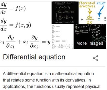
Figure 1. Google information panel that appears on the right side of the page. In this case the search was for “differential equation”. (This image has been shortened a bit.)
The Google KG is extremely general, so it is not as good for all science queries, especially those that clash with popular culture. For example, if you search for the term that describes the surface of a black hole, an “event horizon” you get an image from the bad 1997 movie by that name. Of course, there is also a search engine link to the Wikipedia page describing the real scientific thing. Among the really giant KGs is the Facebook entity graph which is nicely described in “Under the Hood: The Entities Graph” by Eric Sun and Venky Iyer in 2013. The entity graph has 100+ billion connections. An excellent KG for science topics is the Microsoft Academic graph. See “Microsoft Academic Graph: When experts are not enough” Wang et.al. 2019 which we will describe in more detain in the last section of this note. In its earliest form the Google’s KG was based on another KG known as Freebase. In 2014 Google began the process of shutting down Freebase and moving content to a KG associated with Wikipedia called Wikidata. We will use Wikidata extensively below.
Wikidata was launched in 2012 with a grant from Allen Institute, Google and the Gordon and Betty Moore Foundation and it now has information that is used in 58.4% of all English Wikipedia articles. Items in Wikidata each have an identifier (the letter Q and a number) and each item has a brief description and a list of alias names. (For example, the item for Earth (Q2) has alternative names: Blue Planet, Terra Mater, Terra, Planet Earth, Tellus, Sol III, Gaia, The world, Globe, The Blue Gem, and more.) each item has a list of affiliated “statements” which are the “object-relation-object” triples that are the heart of the KG. Relations are predicates and are identified with a P and a number. For example, Earth is an “instance of” (P31) “inner planet” (Q3504248). There are currently 68 million items in Wikidata and, like Wikipedia it can be edited by anyone.
In what follows we will show how to build a tiny knowledge graph for two narrow scientific topics and then using some simple deep learning techniques, we will illustrate how we can query to KG and get approximate answers.
As mentioned above ideal way to construct a KG from text is to use NLP methods to extract triples from text. In a very nice tutorial by Chris Thornton, this approach is used to extract information from financial news articles. If the relations in the object-relation-object are rich enough one may be able to more accurately answer questions about the data. For example, if the triples are as shown in the graph in Figure 2 below
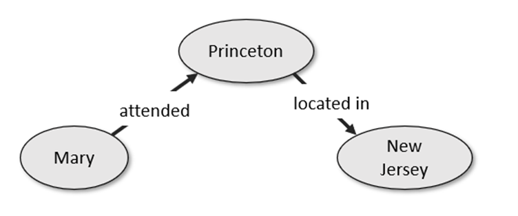
Figure 2. Graph created from the triples “Mary attended Princeton” and “Princeton is located in New Jersey”
one may have a good chance at answering the question “Where has Mary lived?”.There has been a great deal of research on the challenge of building relations for KG. (for example see Sun, et.al) Unfortunately, scientific technical documents are not as easy to parse into useful triples. Consider this sentence.
The precise patterns prevalent during the Hangenberg Crisis are complicated by several factors, including difficulties in stratigraphic correlation within and between marine and terrestrial settings and the overall paucity of plant remains.
Using the AllenAI’s NLP package we can pull out several triples including this one:
[ARG1: the precise patterns prevalent during the Hangenberg Crisis]
[V: complicated]
[ARG0: by several factors , including difficulties in stratigraphic correlation within and between marine and terrestrial settings and the overall paucity of plant remains]
But the nodes represented by ARG0 and ARG1 are not very concise and unlikely to fit into a graph with connections to other nodes and the verb ‘complicated’ is hard to use when hunting for facts. More sophisticated techniques are required to extract usable triples from documents than we can describe here. Our approach is to use a simpler type of relation in our triples.
Building our Tiny Knowledge Graph
The approach we will take below is to consider scientific documents to be composed as blocks of sentences, such as paragraphs and we look at the named entities mentioned in each block. If a block has named entities, we create a node for that block called an Article node which is connected to a node for each named entity. In some cases we can learn that a named entity is an instance of a entity class. In other words, our triples are of the form
(Article has named-entity) or (named-entity instance-of entity-class)
If entities, such as “Hangenberg Crisis”, occur in other blocks from the same paper or other papers we have an indirect connection between the articles.
To illustrate what the graph looks like consider the following tiny text fragment. We will use it to generate a graph with two article nodes.
The Theory of General Relativity demonstrates that Black Holes are hidden by an Event Horizon. Soon after publishing the special theory of relativity in 1905, Einstein started thinking about how to incorporate gravity into his new relativistic framework.
In 1907, beginning with a simple thought experiment involving an observer in free fall, he embarked on what would be an eight-year search for a relativistic theory of gravity. After numerous detours and false starts, his work culminated in the presentation to the Prussian Academy of Science in November 1915 of what are now known as the Einstein field equations, which form the core of Einstein’s famous Theory of General Relativity.
Each sentence is sent to the Google Named-Entity Recognition service with the following function.
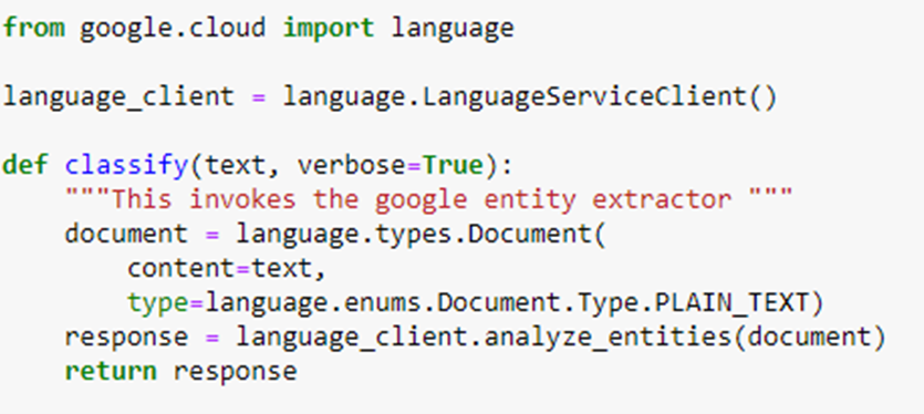
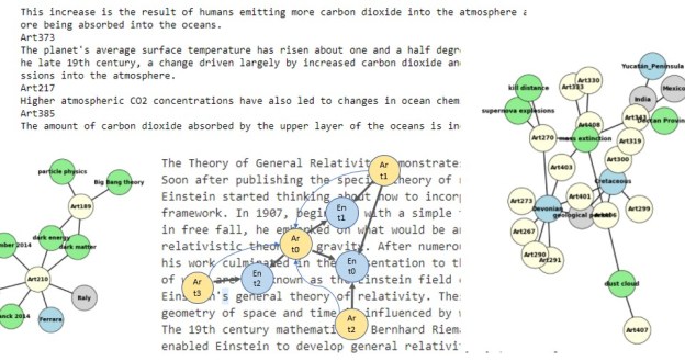
The NER service responds with two types of entities. Some are simply nouns or noun phrases and some are entities that Google NER recognizes as having Wikipedia entries. In those cases, we also use the Wikipedia API to pull out the Wikidata Identifier that is the key to Wikidata. In our example we see three entity node types in the graph. The blue entity nodes are the ones that have Wikipedia entries. The green entities are nodes that are noun phrases. We discard returned entities consisting of a single noun, like “space”, because there are too many of them, but multiword phrases are more likely to suggest technical content that may appear in other documents. These nodes are in green. In the case of the Wikidata (blue) nodes, we can use the Wikidata identifier to find out if the entity is an instance of a class in Wikidata. If so, these are retrieved and represented as gray entities. The first pair of sentences are used to create an article node labeled ‘Art0’. The second pair of sentences are used to form node ‘Art1’.

Figure 3. The rendering of our two-article graph using NetworkX built-in graphing capabilities.
In this case we see that Einstein is an instance of human and an event horizon is an instance of hypersurface (and not a movie). The elegant way to look for information in Wikidata is to use the SPARQL query service. The code to pull the instanceOf property (wdt:P31) of an entity given its wikiID is

Unfortunately, we were unable to use this very often because of time-outs with the sparql server. We had to resort to scraping the wikidata pages. The data in the graph associated with each entity is reasonably large. We have a simple utility function showEntity that will display it. For example,

The full Jupyter notebook to construct this simple graph in figure 3 is called build-simple-graph.ipynb in the repository https://github.com/dbgannon/knowledge-graph.
We will build our tiny KG from 14 short documents which provide samples in the topics climate change, extinction, human caused extinction, relativity theory, black holes, quantum gravity and cosmology. In other words, our tiny KG will have a tiny bit of expertise in two specialized: topics relativistic physics and climate driven extinction.
English Language Queries, Node Embeddings and Graph Convolutions.
Our tiny KG graph was built with articles about climate change, so it should be able to consider queries like ‘The major cause of climate change is increased carbon dioxide levels.’ And respond with the appropriate related items. The standard way to do this is to take our library of text articles stored in the KG and build a list of sentences (or paragraphs) and then use a document embedding algorithm to map each one to a vector in RN for some large N so that semantically similar sentences are mapped to nearby vectors. There are several standard algorithms to do sentence embedding. One is Doc2Vec and many more have been derived from Transformers like BERT. As we shall see, it is important that we have one vector for each article node in our KG. In the example illustrated in Figure 3, we used two sentences for each article. Doc2Vec is designed to encode articles of any size, so 2 is fine. A newer and more accurate method is based on the BERT Transformer, but it is designed for single sentences but also works with multiple sentences. To create the BERT sentence embedding mapping we need to first load the pretrained model.

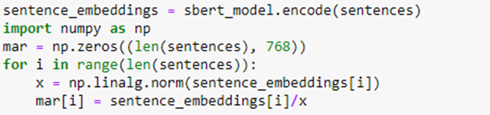
The next step is to use the model to encode all of the sentences in our list. Once that is done, we create a matrix mar where mar[i] contains the sentence embedding vector for the ith sentence normalized to unit length.
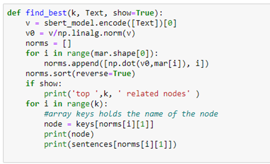
Now if we have an arbitrary sentence Text and we want to see which sentences are closest to it we simply encode the Text, normalize it and compute the dot product with all the sentences. To print the k best fits starting with the best we invoke the following function.
For example, if we ask a simple question:
Is there a sixth mass extinction?
We can invoke find_best to look for the parts of the KG that is the best fit.

Which is a reasonably good answer drawn from our small selection of documents. However there are many instances where it is not as good. An important thing to note is that we have not used any properties of the graph structure in this computation.
Using the Structure of the Graph: A Convolutional Approach.
In our previous tutorial “Deep Learning on Graphs” we looked at the graph convolutional network as a way to improve graph node embedding for classification. We can do the same thing here to use the structure of the graph to augment the Bert embedding. First, for each article node x in the graph we collect all its immediate neighbors where we define immediate neighbor to mean those other article nodes linked to an entity node shared with x. We then computed a weighted sum (using a parameter lambda in [0,1]) of the Bert embedding vectors for each neighbor with the Bert embedding of for x. We normalize this new vector, and we have a new embedding matrix mar2.
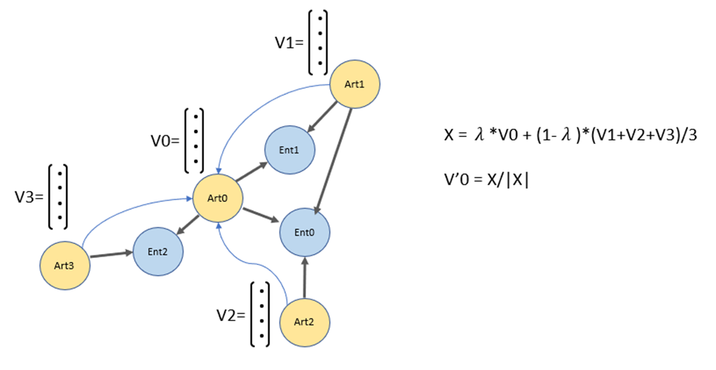
Figure 4. Illustrating the convolution operation
Intuitively the new embedding captures more of the local properties of the graph. We create a new function find_best2 which we can use for question answering. There is one problem. In the original find_best function we convert the query text to a vector using the BERT model encoder. We have no encoder for the convolved model. Using the original BERT encoder didn’t work… we tried.) We decided to use properties of the Graph. We asked the Google NER service to give us all the named entities in our question. We then compare those entities to entities in the Graph. We search for the article node with the largest number of named entities that are also in our query. we can use the convolved mar2 vector for that node as a reasonable encoding for our query. The problem comes when there is no clear winner in this search. In that case, we use the article that find_best says is the best fit and use that article’s mar2 vector as our encoding. Pseudo code for our new find_best2 based on the convolution matrix mar2 is

To illustrate how the convolution changes the output consider the following cases.

The first two responses are excellent. Now apply find_best2 we get the following.

In this case there were 18 article nodes which had named entities that matched the entity in the text: “carbon dioxide”. In this case find_best2 just uses the first returned value from find_best. After that it selected the next 3 best based on mar2. The second is the same, but the last two are different are arguably a better fit than the result from find_best.
To see a case where find_best2 does not invoke find_best to start, consider the following.


Both fail on addressing the issue of “Who” (several people are mentioned that answer this question are in the documents used to construct our KG.). However the convolutional version find_best2 addressed “solve” “field equations” better than find_best.
The process of generating the BERT embedding vectors mar[ ] and the results of the convolution transformation mar2[ ] below is illustrated in Figure 5 as a sequence of two operators.
BertEncode: list(sentences1 .. N ) -> RNx768 GraphConv : RNx768 -> RNx768
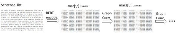
Figure 5. Going from a list of N sentences to embedding vectors followed by graph convolution. Additional convolution layers may be applied.
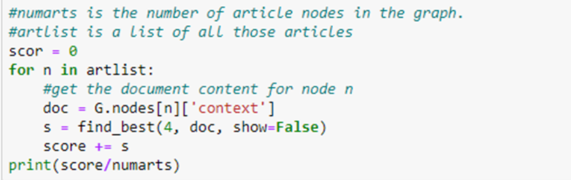
There is no reason to stop with one layer of graph convolutions. To measure how this impacts the performance we set up a simple experiment. This was done by computing a score for each invocation of the find_best function. As can be seen from the results, some of the replies are correct and others are way off. One way to quantify this is to see how far the responses are from the query. Our graph was built from 14 documents which provide samples in the topics climate change, extinction, human caused extinction, relativity theory, black holes, quantum gravity and cosmology. Allocating each of the 14 documents to an appropriate one of 6 topics, we can create have a very simple scoring function to compare the documents in the find_best response. We say score(doc1, docN) = 1 if both doc1 and docN belong to documents associated with the same topic The score is 0 otherwise. To arrive at a score for a single find_best invocation, we assume that the first response is likely the most accurate and we compute the score in relation to the remaining responses
(score(doc1,doc1) + score(doc1, doc2) + sore(doc1, doc3) + score(doc1, doc4))/4.
The choice of measuring four responses is arbitrary. It is usually the case that responses 1 and 2 are good and 3 and 4 may be of lower quality.
The six topics are climate, extinction, human-related extinction, black holes, quantum gravity and cosmology.
Notice that we are not measuring the semantic quality of the responses. We only have a measure of the consistency of the responses. . We return to the topic of measuring the quality of response in the final section of the paper. The algorithm to get a final score for find_best is to simply compute the score for each node in the graph.
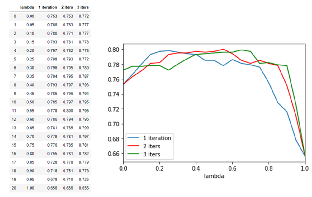
We do the same for find_best2 for different layers of convolution. As can be seen from the chart below one convolution does improve the performance. The performance is peaked out at 3 convolutional layers.

Recall that the convolution operator was defined by a parameter lambda in the range 0 to 1. We also ran a grid search to find the best value of lambda for 1, 2 and 3 convolutional layers. We found a value of 0.75 gave reasonable results. (note that when lambda = 1 the layers degenerate to no layers.)
Plotting the Subgraph of Nodes Involved in a Query
It is an amusing exercise to look at the subgraph of our KG that is involved in the answer to a query. It is relatively easy to generate the nodes that connect to the article nodes that are returned by our query function. We built a simple function to do this. Here is a sample invocation.

The resulting subgraph is shown below.

Figure 6. Subgraph generated by the statement “’best-known cause of a mass extinction is an Asteroid impact that killed off the Dinosaurs.”
The subgraph shown in figure 6 was created as follows. We first generate an initial subgraph generated by using the article nodes returned from find_best2 or find_best and the entity nodes they are connected to. We then compute a ‘closure’ of this subgraph by selecting all the graph nodes that are connected to nodes that are in the initial subgraph.
Looking at the subgraph we can see interesting features. An amusing exercise is to follow a path from one of the nodes in the graph to the other and to see what the connections tell us. The results can form an interesting “story”. We wrote a simple path following algorithm.
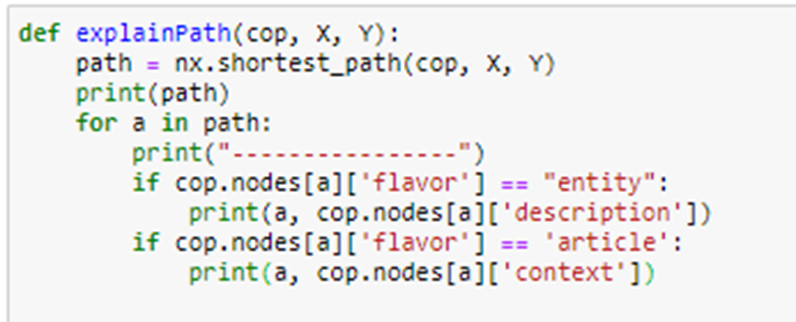
Invoking this with the path from node Art166 to Art188

gives the following.

Trying another path

Yields the following

There is another, perhaps more interesting reason to look at the subgraph. This time we use the initial subgraph prior to the ‘closure’ operation. If we look at the query

The results include the output from find_best2 which are:

You will notice only 2 responses seem to talk about dark energy. Art186 is related, but Art52 is off topic. Now, looking at the graph we see why.

Figure 7. Subgraph for “What is dark energy”
There are three connected components, and one is clearly the “dark energy” component. This suggests that a further refinement of the query processing could be to filter out connected components that are “off topic”.
We conducted a simple experiment. In calls to find_best2(4, text) we searched the ten best and eliminated the responses that were not in the same connected component as the first response. Unfortunately this, sometimes resulted in fewer than k responses, but the average score was now 83%.
Conclusion
In this little tutorial we have illustrated how to build a simple knowledge graph based on a few scientific documents. The graph was built by using Google’s Named Entity Recognition service to create simple entity nodes. Article nodes were created from the sentence in the document. We then used BERT sentence embeddings to enable a basic English language query capability to pull out relevant nodes in the graph. Next we showed how we can optimize the BERT embedding by apply a graph convolutional transformation.
The knowledge graph described here is obviously a toy. The important questions are how well the ideas here scale and how accurate can this query answering system be when the graph is massive. Years of research and countless hours of engineering have gone into the construction of the state-of-the-art KGs. In the case of science, this is Google Scholar and Microsoft Academic. Both of these KGs are built around whole documents as the basic node. In the case of the Microsoft Academic graph, there are about 250 million documents and only about 36% come from traditional Journals. The rest come from a variety of sources discovered by Bing. In addition to article nodes, other entities in the graph are authors, affiliations, concepts (fields of study), journals, conferences and venues. (see “A Review of Microsoft Academic Services for Science of Science Studies”, Wang, et. al. for an excellent overview.) They use a variety of techniques beyond simple NER including reinforcement learning to improve the quality of the graph entities and the connections. This involves metrics like eigencentrality and statistical saliency to measure quality of the tuples and nodes. They have a system MAKES that transforms user queries into queries for the KG.
If you want to scale from 17 documents in your database to 1700000 you will need a better infrastructure than Python and NetworkX. In terms of the basic graph build infrastructure there are some good choices.
- Parallel Boost Graph Library. Designed or graph processing on supercomputers using MPI communication.
- “Pregel: A System for Large-Scale Graph Processing” developed by Google for their cloud.
- GraphX: A Resilient Distributed Graph System on Spark.
- AWS Neptune is fully managed, which means that database management tasks like hardware provisioning, software patching, setup, configuration, and backups are taken care of for you. Building KG’s with Neptune is described here. Gremlin and Sparql are the APIs.
- Janus Graph is an opensource graph database that is supported on Google’s Bigtable.
- Neo4J is a commercial product that is well supported, and it has a SQL like API.
- Azure Cosmos is the Azure globally extreme-scale database that supports graph distributed across planet scale resources.
If we turn to the query processing challenge, the approach we took in our toy KG, where document nodes were created from as few as a single sentence, it is obvious why the Microsoft KG and Google Academic focus on entire documents as a basic unit. For the Microsoft graph a variety of techniques are used to extract “factoid” from documents that are part of concepts and taxonomy hierarchy in the Graph. This is what the MAKES system searches to answer queries.
It is absolutely unclear if the convolutional operator applied to BERT sentence embedding described here would have any value when applied to the task of representing knowledge at the scale of MAG or Google Scholar. It may be of value in more specialized domain specific KGs. In the future we will experiment with increasing the scale of graph.
All of the code for the examples in this article is in the repository https://github.com/dbgannon/knowledge-graph.
