
This is a small tutorial supplement to our book ‘Cloud Computing for Science and Engineering.’
Introduction
Machine learning has become one of the most frequently discussed application of cloud computing. The eagerness of cloud vendors to provide AI services to customers is matched only by their own interest in pushing the state of the art for their own internal use. In Chapter 10 of our book we discussed several “classical” machine learning algorithms and we introduced some the methods of deep leaning using three different toolkits: MXNet, Tensorflow and CNTK. We also described several cloud AI services available on AWS and Azure. However, one topic that we did not address at all was the training of neural nets that use the parallel computing capabilities available in the cloud. In this article we will do so using another deep learning toolkit, PyTorch, that has grown to be one of the most popular frameworks.
In the simple tutorial that follows, we will first describe PyTorch in enough detail to construct a simple neural network. We will then look at three types of parallelism that can be used while training a neural net. The easiest to use is GPU parallelism based on Nvidia-style parallel accelerators. We will illustrate this with an example based on the PageRank algorithm. Next, we will consider distributed parallelism where multiple processes collaborate and synchronize around the training of a single neural network. The obvious extension of this is to use multiple processes, each with a GPU to accelerate performance. Finally, we will briefly describe the use of multiple GPUs in a single thread to pipeline the training of a network.
A Tiny Intro to PyTorch.
PyTorch 1.0, which was open sourced by Facebook in 2018, has become one of the standards for deep learning. The website is well documented with some excellent tutorials, so we will not duplicate them here. However, to make this readable, we will introduce some basic Torch ideas here and refer to the tutorials for in-depth learning. PyTorch is deeply integrated with Python. As with all deep-learning frameworks, the basic element is called a tensor. At a superficial level, a PyTorch tensor is almost identical to a Numpy array and one can convert one to the other very easily. The primary difference is the set of operators possible on a PyTorch tensor and the fact that a tensor can retain the history of operators that created it. This history can be used to create derivative and gradients that are essential for training neural networks. We will return to this property later, but first let’s look at some basic tensor properties.
In the example below we create a Numpy array of 5 rows and 3 columns with 1’s for each element and use it to create a PyTorch tensor.

PyTorch is extremely flexible. For example, we can create a tensor from a python list of values and use this tensor to create a diagonal matrix.

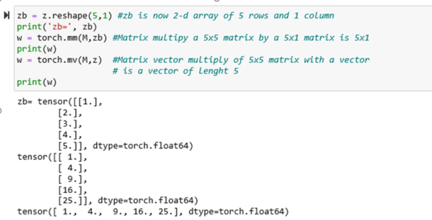
Operations such as matrix-matrix multiply (torch.mm()) and matrix-vector multiply (torch.mv()) are based on reasonable standard algebraic rules. We will illustrate this with our vector z and matrix M from above. Matrix-Matrix multiply requires 2-d tensors, but we can reshape our vector into a 2-d array. Once it is 2-D we can multiply it by our matrix. Or we can do a matrix vector multiply using M and the original 1-d vector z. The result of the matrix multiply is a 2D 5×1 matrix. The matrix vector multiply yields a 1-d vector.
Regular multiplication and addition are different. if you multiply a tensor of the form [a, b]*[c,d] the result is the elementwise product [ac, bd]. In the case one of the operands is a matrix the result is shown below. Let’s start with M and add 1 to each element then do a point wise multiply.

These are only a few of the PyTorch operators, but they are sufficient for describing the material that follows.
Using the GPU
If you have access to a server with a GPU, PyTorch will use the Nvidia Cuda interface. Working with the GPU is not very elegant, but it is simple and explicit. If you have a server with three GPUs, they are named “cuda:0”, “cuda:1”, ‘’cuda:2”. To do computation on the GPUs you must move all the associated data explicitly to the GPUs. To create a tensor on “cuda:1” one writes

If there is only one GPU, the name “cuda” is sufficient. To move a tensor to the GPU from the CPU memory to the GPU you write

Moving a GPU resident tensor back to the CPU memory one uses the operator .to(‘cpu’).
GPU parallelism: The PageRank algorithm
To illustrate the programming and behavior of PyTorch on a server with GPUs, we will use a simple iterative algorithm based on PageRank. It is not necessary to understand the derivation below because we will only be concerned with the performance results. But, for completeness we describe it anyway.
PageRank is an algorithm introduce in 1996 by Larry Page and Sergey Brin to rank web pages in their early version of the Google search engine. The rank can be considered the relative importance of a page. Consider a graph G of N nodes. Let link(i) by the set of nodes that point to node i. And let out(j) be the number of links out of node j. The formula for computing the rank Pr(i) for each node i in g is given by

Where the scalar d is called the damping factor and it is a number between 0 and 1. This formula is for the special case that there is at most one link from a node to another. (You can read the Wikipedia article to learn more about this equation.) We can recast this in matrix algebra terms as follows. Let G(I,j) be the adjacency matrix of G , i.e. G(i,j) = 1 if there is a link from j to i in G and zero otherwise. Let Out be a diagonal matrix with the value 1/out(j) on the jth diagonal element when out(j) is not zero and zero otherwise. The formula above can be written in matrix form as

Where Pr is the vector of Pr(j)’s and the “dot” is matrix or vector multiply depending on the association (G*Out)*Pr or G*(Out*Pr). (As we shall see the choice can make the difference in computational cost substantial.) As you can see, Pr is closely related to an eigenvector of G*Out. In fact if d = 1, it is an eigenvector. To compute it, we can turn this into a simple iteration

Fortunately, this converges to the “principle eigenvector” solution rather rapidly. We will use this to compare GPU computation to regular CPU computing.
Our goal is to demonstrate how to do PyTorch computation on the GPU and compare the performance to running on the cpu and we will use the iterative page rank algorithm to do this. To build a sample network and adjacency graph, we will use the NetworkX python package to create a slightly modified random (binomial) Erdős-Rényi graph (see this page for details). The graph was modified so that every node has at least one outgoing node. To use this graph with PyTorch, we use the lovely DGL library from library from NYU and Shanghai by Minjie Wang, Jake Zhao, Prof. Zheng Zhang and Quan Gan.
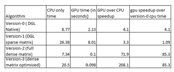
We considered 4 different implementations of the page rank algorithm and run them on a single cpu and a single GPU. (We describe multiple CPUs and GPUs in the neural net example in the next section.) Version-0 is one that is described in the DGL documents and we will not reproduce it here because it uses many of the features DGL that are not important for our discussion. We ran it (and the others) on AWS with a p2.xlarge server which has a single NVIDIA K80 GPU. The graph we created and tested with has N= 10000 nodes. We used K=200 iterations and a value of d=0.85. In all our tests the results converged to the same result within roundoff error. (The complete source for these examples and experiments are available in gitub.)
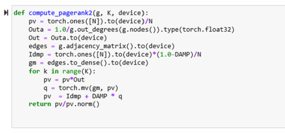
Version-1 of the algorithm uses the fact that the DGL library of a sparse graph interoperates fully with the PyTorch library. Hence the PyTorch matrix-matrix multiply and matrix-vector multiply work when one of the arguments is a sparse matrix representation of our graph. The core of the algorithm is shown below. This function takes the DGL representation of the graph, the number K of iterations and a parameter device that is either the text “cuda” or “cpu”.

Our pv vector is created as all ones on the selected device. Lines 2 and 4 are DGL operators. In line 2 and 3 we construct the Out array as a Nx1 matrix. (To simplify things, there is no divide-by-zero here because of the modification to the graph above.) In line 4 we extract the adjacency matrix as edges. Idmp is a Nx1 matrix that is (1-DAMP)/N for each element where DAMP is the value for d. It is important to notice we are using the sparse representation of the matrix edges in the matrix-matrix multiply.
Version-2 is almost identical to Version-1 except that we convert the edges matrix to a dense form prior to executing the loop as shown below.
Notice that in version-2 above there is a pointwise product pv*Out inside the loop prior to the matrix vector multiply. Because of the associativity we described above, we can move Out outside the loop and convert it to a diagonal matrix and multiply it with gm as shown in version-3 below.

The performance of all four of these Pagerank algorithms is shown in the table below. Each algorithm was run with the parameter device set to “cpu” and “cuda”. As one can see the CPU-only time for version-0 is the second best, but it does not profit from the GPU as much as version 2 and 3. Version-1 is not competitive at all. It is most interesting to note the difference between Version-2 and Version-3. The behavior can be explained easily enough. Replacing K (200) vector point products with an NxN matrix-matrix multiply is not very smart if N=10000 and matrix multiply is an O(N3) algorithm. The surprising thing is how well the matrix multiply and matrix vector multiply are optimized on the GPU. In these cases speed-ups of 2 and 3 orders of magnitude are not uncommon. Unfortunately, the DGL sparse matrix-vector multiply in Version-1 is not as well optimized.
This example illustrates that the GPU is capable of substantial performance improvements in a matrix-vector computation in PyTorch. The source code for this example as a Jupyter notebook is in github along with the other examples from this chapter. Now we return to Neural nets.
Neural Net training with the PyTorch and the GPU
One of the advantages of frameworks like PyTorch is how easy it is to build a neural network. To illustrate this point, we will build network that takes real, scalar values for x and learns to compute an arbitrary function f(x). To do this we will train the network by selecting a sequence of values xi in an interval [a, b] for i=0,….N and supplying it with f(xi). The result will be a network that is very good at computing f(z) for any z in [a, b]. Of course, this is not as exciting as deep neural networks that take inputs x that represent an image and f(x) is a description of the content of the image, but the concept is exactly the same. The only difference is that when x is a 64×64 pixel color image it is not a single real number but a vector of real numbers in a space of dimension 64x64x3, which is pretty big. For our purposes, dimension = 1 is sufficient.
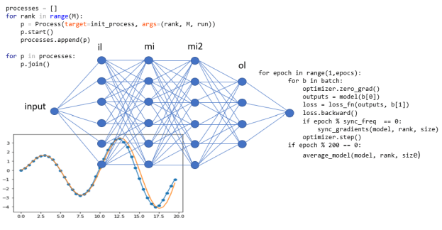
We will construct the network as four layers with an input layer of size 80, two middle layers of size 80 and an output layer of size 40. (80 and 40 are somewhat arbitrary here. There was no attempted to find optimal values.) These are linear layers so the connections to the previous ones are complete as illustrated in the figure bellow.

This is an extremely simple type of network that has enough layers we can say it is “deep-ish”. (A really deep network for a serious imaging problem will have around 50 layers.) The PyTorch code to specify this network is shown below.

The network is created as a subclass of torch.nn.Module and each instance contains instances of our four layers. It also contains an instance of a rectified linear operator defined by ReLU(x) = max(0, x). The method forward(x) defines how an input scalar tensor x is processed through the network. Each linear layer takes a vector of length 80 and produced an output of the same shape. However, we apply the ReLU operator to the input of all interior nodes except the input layer. ReLU is an “activation” function that decides when a “neuron” turns on (in this case when the input is positive). In more mathematical terms, this allows the network to behave like an arbitrary continuous non-linear function. Without it, the network is a completely linear transformation. (The mathematical proof if this “universality” can be seen in the early work of George Cybenko and others.)
To train the network we will provide inputs and target values and adjust the parameters that define the links. More specifically each layer has an associated matrix W and offset vector b. The forward(x) function computes the following. It is the training step determines the “best values” of the Ws and bs.

We use the standard least squares error between the values for Out and the target data to determine “best values” and we use stochastic gradient decent to do the optimization. But to do this we need to compute the gradient of Out with respect to each of the Ws and bs. As mentioned previously, torch tensors are capable of recoding the history of their creation and we can work backward to compute the derivate of values computed with them. To force a tensor to begin a chain of computations we create it with the flag requires_grad=True as in the example below.

Then to compute the gradient of out with respect to x we invoke the backward() operator as follows.

To verify this, we can get out the old derivative chain rule and compute this by hand as

and plug in the numbers to get.

You don’t want to compute the gradient of our neural network output by hand. Let Backward do it automatically.
Training the network is now easy. We first gather together values for the input and target. In our trivial test case we will use the input to be numbers from the interval [0.0, 20.0] and the function is f(x) = sqrt(x)*sin(3.14*x/5.0).
The training loop, in its simplest form, is shown below with an SGD optimizer and the mean squared error loss function. The optimizer is given the learning rate of 0.001. Like our choice of 80 for the size of the network layers, this was somewhat arbitrary, and it worked.

Running this with various parameters to make it converge, one can test the network by providing values for the input and recoding the output. Plotting the result (blue) against the target function (orange) one can see the convergence.

A more conventional approach to the training is to divide the input and target vectors into small “mini-batches” and passing each mini-batch through the loss-gradient-generation-optimization step independently. This generates substantially faster convergence rates. As we shall see, this independence also allows us to compute them in parallel and merge the results later.
Basic distributed computing with PyTorch
We have already described how PyTorch exploits GPU parallelism. If a server has multiple cores or if you have a cluster of servers available, it is also possible to use MPI-like message passing style to coordinate multiple thread of computation. One must create a master process that forks off child processes that do the work. One way to do this that works for Jupyter notebooks but not GPUs looks like the following.

The Process function creates an instance of a processes that is passed an initialization function and an identifier “rank”, the total “size” of the collection of threads and a function “run” that will be invoked once the initialization is complete. The init_process is run on each created thread and it initializes a communication backend that the spawned processes share. In the case above it is called “gloo” and it works for a single multicore server. However, one can also MPI or NCCL. If you have a cluster with Infiniband, NCCL is the one to use. We will not discuss NCCL here. See this page for more details.
If you are running on a multi-GPU system you must use a different method to launch the processes from a python program and not a Jupyter notebook. The program looks like

We will call this the mp.spawn(…) version of the launch program. It is run from the command line and not Jupyter.
In this case the run(rank, size) function must call setup(rank, size) first then then clean-up later. The Github site has three programs: distributed_learn_multicore-final.ipynb which illustrates the training of our neural net using the first method described above, distributed_lean_gpu-final.py which uses a server with 8 GPUs to do the training, and distributed_local.ipynb which illustrates the basic communication primitive. We discuss these basic communication methods next and then give some performance results of the distributed learning cases.
We illustrate the communication system with three different “run” function examples. The first one illustrates basic MPI-style message passing. This one simply passes a tensor from process 0 to 1 and then from 1 to 2 and then to 3. Each time it adds 1 to the tensor.

The output from each process is routed to the master and is what you would expect (except the order in which the lines are received are random). Running this with P=3 child process gives the result below.

PyTorch also support many standard collective communication routines. For example, to compute the sum of elements from each process we use a reduction operator. The input is a Torch data structure of identical shape on each process. The reduction overwrites the input tensor with the sum of the corresponding elements of all processes.

In this case process 0 has a scalar tensor with value 1, process 1 has a tensor with value 2 and process 2 has a tensor with value 3. The output of the reduction is

The notebook distributed-local.ipynb has complete code for these communication examples.
Parallelizing the Training of our Neural Net
In this section we will describe the results of using two different approaches to parallelize the training phase of our demo neural network. The first method will be to use a server with multiple GPUs. The second method use multiple cores on a multicore server without GPUs.
The multi-GPU method
In this case we are using an AWS p2.8xlarge server which has 8 NVIDIA K80 GPUs and 16 cores with 488 GBytes of memory. Because we are using GPUs we have to use the mp.spawn( … ) version of the launch program described above. The network is the same one we described above. We created a dataset of size 80000. The variable M is the number of processes and BS is the batch size. A function batchtodev(rank, device) delivers a list of 80000/(M*BS) unique batches of data to the process identified by the local variable rank. The run function now takes the form
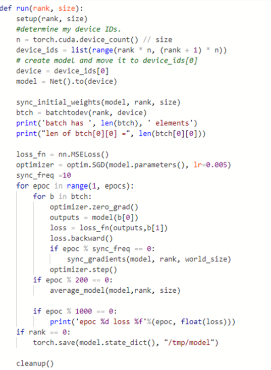
The initialization function setup(…) is described with the mp.spawn(…) code described above. The way in which the GPUs are allocated to threads is a bit confusing. It is designed so that if you have D GPUs and M threads, each thread is assigned a unique list of D/M GPUs. We only use the first GPU on the in each thread.
The training loop in this version now iterates through each of the elements in the batch list for each epoch. There is function sync_init_weights( ), a conditional controlling a periodic call to sync_gradients( ) and every 200 epochs we call a special function average_mode( ). Sync_init_weights() uses a simple broadcast to copy the initial random-state network to the other threads. While it is possible to allow each thread to create its own converged model they will not converge to anything much because each thread has only one fraction of the full data set. We need a way to periodically tie the independently evolved models together. That is done every 200 epochs with the call to average_model( ) which uses a global reduce sum operation. See distributed-lean-gpu-final.py for the details of these functions.
Another approach to blending the results of multiple training threads is to average the gradients from each parallel set of mini-batches before the optimizer step. This is what the function sync_gradients( ) accomplishes. But doing this every mini-batch step adds a great deal of thread synchronization overhead. Is it really necessary to do this every step? Doing it often does improve the rate of convergence, but what happens if we do it periodically? In the table below, we run the training for our network of size N=80000 with BS = 1000 until the loss is below 0.05. This is done for doing it every mini-batch step, then for every 2, 4,10 and never mini-batch steps and finally “never” to see what happens if we only rely on average_model().
| frequency | 1 | 2 | 4 | 10 | never |
| time | 330 | 183 | 136 | 99 | 88 |
| loss | 0.039 | 0.05 | 0.04 | 0.025 | 0.03 |
| Epochs x 1000 | 4 | 6 | 6 | 7 | 8 |
| total time | 1320 | 1098 | 816 | 693 | 704 |
This version was run on an Intel core-i7 with M = 4 threads using the no-GPU method (described in the next section). The results from run-to-run vary greatly because of the randomness in the processes, but it was clear that doing it every mini-batch step produced excellent convergences, but at high cost. It must also be noted that the penalty for the overhead depends on the size of the network (which equals the size of the gradient) and many other factors.
Running on 8 GPUs on one server.
Turning to the performance of our training code on the AWS 8-cuda core server, we ran the same configuration (N=80000, BS=1000) but rather than compare convergence rates, we ran it for 10000 epochs for 1 GPU, 2 GPUs, 4 GPUs and 8 GPUs. At 10000 epochs they were all converged, but using the same number of epochs means that the total amount of work was the same in each case. The results are below. If we compare the performance of 1 GPU to 8 GPU we realize a speed-up of 6.74.
| gpus | 1 | 2 | 4 | 8 |
| elapsed time | 934 | 489 | 249 | 139 |
| cuda speed-up | 1 | 1.91 | 3.75 | 6.74 |
Our test case is extremely small. Much greater performance gains are possible with greater numbers of GPUs when larger problems are used.
The no-GPU method
This version uses multi-core servers without GPUs. We ran this on an AWS c5n4xl server with 32 gig of memory with 8 real cpus (16 virtual cpus). The network is the same one we described above. We created a dataset of size 80000. The variable M is the number of processes and BS is the batch size. As before, A function batchtodev(rank, ‘cpu’) delivers a list of 80000/(M*BS) unique batches of data to the process identified by the local variable rank. The run function now takes the form

In this case we had a surprise. Using PyTorch multiprocessing and increasing the number of processes thread did not increase performance. In fact, it got worse! The table below is for 8, 4, 2 and 1 processes with the best performance for 1 process. We also give the results for the Intel Core i7 running ubuntu in a Docker container.
| processes | 8 | 4 | 2 | 1 |
| cpu elapsed time | 4801 | 3003 | 1748 | 1403 |
| cpu speed-up | 1 | 1.7 | 1.8 | 2 |
| cuda/cpu speedup | 5.1 | 6.1 | 7 | 10.1 |
| corei7-docker | 1282 | 1274 | 1064 | 1151 |
There is an interesting explanation for this behavior. The fact is that for PyTorch 1.3.0 and 1.3.1, the basic neural net functions (model evaluation, backward differentiation, optimization stepping) are all optimized to use all available cores. So in the case of one process thread, all 16 cores are dividing the work. In the case of 2 processes, there are 2 groups of 8 cores each working and the multithreading is pure overhead. In all cases all cores are busy and the number of process threads only adds overhead. This was verified by running the Linux “top” command.
Of course, if you run this on a cluster of multicore servers using the MCCI or MPI runtime, one can expect different behavior. There have been numerous studies of the parallel training performance. One we like is Parallel and Distributed Deep Learning , by Vishakh Hegde and Sheema Usmani.
Model Parallelism
In the examples above we have used multiple copies of a neural net running on separate threads and then merged the results together. As we have shown this works with multiple GPU on a single server, but without a GPU, we did not get performance that beat the native PyTorch built-in multi-core parallelism.
There is another approach to parallelizing the training and model evaluation computation that is in some sense, orthogonal to the method we described above. This can be very valuable if the model does not fit in a single GPU memory. One can slice the network so that the first few layers are in one GPU and the rest are in a second GPU. Then you can feed inputs into the first, transfer the data from the last layer in the first GPU to the first layer in the second GPU. Of course doing this, by itself, does not buy you any parallelism: one GPU is idle while the other is work. However, one can “pipline” batches through the model. In this way batch0 goes to GPU0 and then to GPU1. A soon as batch0 clears GPU0, push batch1 to GPU0 while GPU1 is working on batch0. You need to accumulate the set of batches at the end and them concatenate them together as described in this PyTorch best practices tutorial.
However, one can do even more with pipelining as part of parallelization. The back propagation algorithm is based on computing the gradients of the error from the last layer to the first layer it is possible to push to gradient back through our pipeline of GPUs. A group at Microsoft Research, CMU and Stanford has pushed this idea and produced a very nice paper at SOSP19. The figure below, from that paper, illustrates the idea. You distribute the layers among the GPUs (using data parallelism for very dense layers) and pipeline batches as described above. Then you also let the back propagation push back up the pipeline. After a startup, there is plenty of work to fill the available gpu slots. However, to get this to work requires a sophisticated resource scheduler and care must be taken to make sure the model is consistent and converges correct. Read their paper. It is very nice.

