
Abstract
A persistent problem when using deep neural networks in production is the speed of evaluating the network (known as inference) on a single input. While neural network inference has ample opportunities for using parallelism to gain speedup, these techniques are not as easy to exploit as when training the network. In this short report we will look how several new system/chip designs from companies like Groq, Celebras, Graphcore and Samba Nova are approaching the inference performance problem and we will also explore the software challenge in compiling Neural Nets to run on this parallel computer hardware.
Why is Inference Harder to speedup than Training?
Training Deep learning systems require vast computational resources and data. Fortunately, the algorithms used for training are highly parallelizable and hardware that supports either data parallel and/or highly multithreaded execution can make a huge difference in the training time. In a previous post, we described how simple GPUs and clusters of CPUs can be used to train networks. However, once a network has been trained it must be deployed so one can use it to make inferences. Making an inference involves taking a single input (an image, query or sound clip) and pushing it through the many layers of the network. The trained model may be hosted in the cloud to support image identification or search, or to do natural language translation or question answering. Doing this fast for on-line applications is essential as the load on the application increases. The speed of inference is also critically important in robotics applications such as self-driving vehicles or controlling complex critical hardware which may involve life-support.
While the inference process still involves operations that can be parallelized, the challenge in using this parallelism to gain performance is different than it is when training the network. The reason that this is the case is easy to understand. The metric of performance for inference is latency (the time it takes to push an item through the network) while the metric of performance for training is throughput (the volume of training data per second that you can manage). Training a network involves pushing batches of training data through the pipeline of network layers. GPUs are effective when you can reuse data that has already been loaded into their local memories. Evaluating a batch of input data allows the GPU to load the layer weights once and reuse them for each item in the batch.
It is a well-known fact of life in high performance computing that the latency involved moving data is a performance killer unless you can hide that latency by using your hardware to do other useful computation. Because inference has fewer opportunities to reuse data, the best way to reduce inference latency is to reduce the amount or cost of data movement.
The new architectures we will look at all use extraordinary amounts of parallelism, but they also depend very heavily on compilers that can translate the neural network designs into the low level code and optimized data movements that will achieve the performance goals. In fact most, if not all, of the systems here were co-design efforts involving the simultaneous planning for the hardware and software. Hence as we present hardware details, we will need also to describe the compiler and runtime. The last section of this report will focus on the general challenges of compilers for this class of computing system.
Hardware Advances
In the following paragraphs we will outline the advanced deep learning processor designs that are now coming on the market. While they all address the issues of training and inference, there are several that has put the issue of inference performance as a prime design objective. The descriptions below vary greatly in the level of detail. The reason for this is that some are still a work in progress or highly proprietary. For example, all we know about the Huawei Ascend 910 is that it “performs much better than we expected”.
Groq
Groq.com is a Silicon Valley company co-founded by Johnathan Ross who was on the team that designed the Google Tensor Processing Unit. The Groq Tensor Streaming Processor (TSP) is very different from the other systems which rely on massive scale multi-core parallelism. Instead the TSP can be classified as a Very Long Instruction Word (VLIW) single core, single instruction stream system. The design is very unusual but there is a good description in the Linley Group Microprocessor Report January 2020. We will only give a capsule summary here.
The TPU is a type of systolic processor in that it has horizontal data flows with instructions streaming from the main issue engine down through 20 data layers called superlanes. Each Superlane is composed of 16 parallel lanes of 8 byte wide data paths. The superlanes have blocks for Matrix accumulators, transpose and permute operations and vector ALUs as shown in Figure 1 below. Note that memory is imbedded directly in the superlanes. Notice also that each superlane has is duplicated around a central axis so data moves between units in both directions
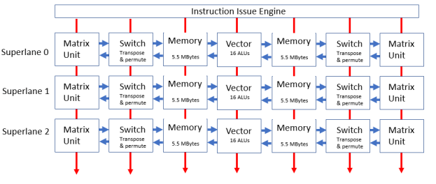
Figure 1. Groq Architecture.
Instruction issue is also systolic. The first instruction is executed on superlane 0 in one cycle. In the next cycle that instruction is executed on superlane 1 while the 2nd instruction is executed on superlane 0. In the next cycle the first instruction is executed on superlane 2, the 2nd instruction is now on superlane 2 and the 3rd instruction is on superlane 0. So, in 20 cycles an instruction has been executed on all superlanes and each subsequent instruction is complete on all superlanes, etc. (Note: this description may not be totally accurate. We do not have the detailed Groq technical specs.)

Figure 2. Groq TSP
The Groq TSP is designed to deliver a 1000 trillion operations per second and live up to a major design goal: on the Resnet-50 deep learning model it delivers 20,000 inferences per second with a latency of 0.04ms on a batch size of 1.
A big challenge in creating a system like the Groq TSP is building a compiler that can generate an efficient instruction stream to keep all that hardware busy. Because there are no caches, locality is not an issue and advanced architectural features like prefetch and branch prediction are not needed, so the computation is completely deterministic, and performance is completely predictable. We will return to the compiler issues below.
Habana Goya
Habana Labs was one of the first to introduce a fast inference processor. In 2018 they announced the Goya processor. By the end of 2019 they were acquired by Intel. The Goya architecture has an array of Tensor Processor Core (TPC) compute engines which are VLIW single-instruction-multiple-data processors. It also has a general matrix multiply engine. The TPC engines have local memory but there is a fast, shared static RAM.
One very interesting thing about the Habana design team is their work with Facebook on the Glow compiler back end for Pytorch. More on that later.
Alibaba Hanguang 800
Another newcomer to the race for faster inference is the Alibaba Hanguang 800. Alibaba is not planning on selling this new chip and it is intended solely for internal use in its cloud servers. There is very little that is published about its internal architecture. In the table below we see some interesting performance numbers including one that indicates that the Alibaba system has better inference performance than the Groq TSP. However, we do not know if this IPS number is for a batch size of 1.
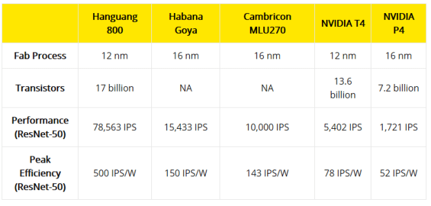
Figure 3. From https://www.techarp.com/computer/alibaba-hanguang-800-details/
A Digression about Compilers, ResNet-18 and ONNX.
Before we continue discussing interesting new architectures, it is helpful to stop and discuss some general issues related to the compilers and benchmarks.
One of the big problems you encounter when writing a compiler for a new architecture is that there are several very good deep learning frameworks that are used to build deep neural networks. These include MxNet, Caffe, CNTK, Tensorflow, Torch, Theano, and Keras. One could write a compiler for each, but, given that they all build very similar network models, it makes sense to have a “standard” high-level, graph intermediate form that captures the properties of a large fraction of all neural nets. Then, if third parties build translators from the high-level frameworks to this intermediate form, the chip architect’s job is half done: all they need to do is write a code generator mapping that intermediate to their architecture.
The Open Neural Network Exchange (ONNX) may become that standard intermediate form. Originally developed by Microsoft and Facebook, it has been taken over as a community project involving 20 companies. While we do not know how Groq, or some of the other hardware companies described here, are building their proprietary compilers, looking at ONNX as it relates to a real example can give a clue of how compilers like these do work.
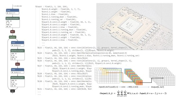
In the last three hardware descriptions, performance number were often cited in terms of ResNet-50. Resnet is one of a family of very deep convolutional neural networks. Originally presented by He, Zhang, Ren and Sun in their 2015 paper, they describe a clever way to improve the ability to train very deep networks. You can think of each level of a deep neural network as learning more subtle and abstract features of the training images than were detected by the previous layers. A residual network is one where you “subtract” the features discovered by previous layers so the following layers can work on learning the properties of the residual. Doing this subtraction is a way to focus the learning on what remains and helps solve a problem known as the vanishing gradient that makes it hard to train very deep networks. Mathematically If your training goal is to learn a function H(X), then the residual at some layer is F(X) = H(X)-X. Hence we want the following layers to learn F(X)+X to recover H(X). Creating F(X)+X in the network is easy and it is shown in Figure 4.
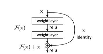
Figure 4. From Zhang, Ren and Sun in their 2015 paper.
We can construct such residual network with Torch or TensorFlow and then we can look at the ONNX intermediate. In Torch, the code is summarized below. (The complete code is in a Jupyter notebook that accompanies this post.) There are two networks. One is the residual block as illustrated in Figure 4 above and the other is the full model that incorporates a sequence of residual blocks.
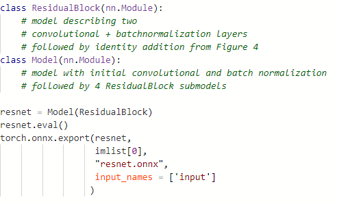
In the image above, we created an instance of the model as “resnet” and then set it to the eval() state. Using the Torch built-in ONNX export operator we can save a copy of the model in the file resnet.onnx. Doing so gives an output like Figure 5 below. On the right we have fragments of the ONNX intermediate code and on the left, a graph that is generated from the ONNX code with a tool called netron. What is shown here is only a small part of the ONNX graph. The top is just a list of all the model variables. Following that we have actual code for the graph.
The ONNX exporter will build the graph from the internal Torch model. There are two ways in which it does this. One is to directly “unroll” the graph by interpreting the execution of the forward(input) eval operator. In some cases, if the definition of the model contains conditionals, it will insert conditional code in the graph, but these are rare cases.
In this case the code consists of an initial convolutional layer followed by a batch normalization which is based on the mean and variance of previously seen batches. This is followed by the first instance of the Residual block model.
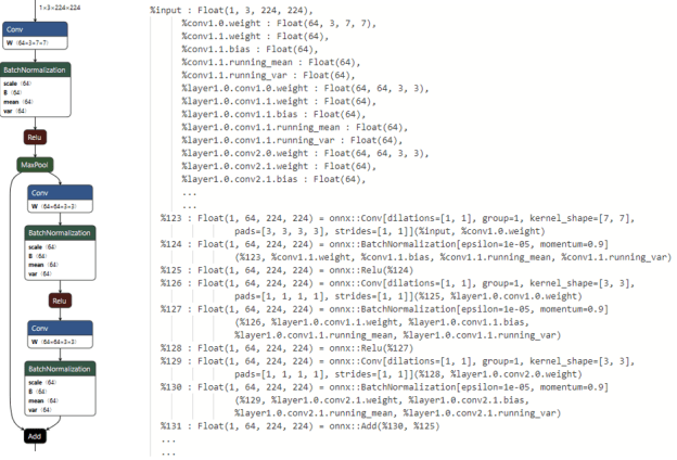
Figure 5. Fragment of the ONNX output for the Resnet18 model.
As you can see, the ONNX graph consists of nodes that are parameterized operators with inputs that are the model tensors and they produce one output that is a well-defined tensor. Generating code for a specific architecture can be a simple as building well-tuned native versions of the ONNX operators and then managing the required data movement to ensure the input tensors are in the right place at the right time for their associated operation nodes. On the other hand, there are a number of important optimization that can be made as we “lower” the ONNX graph to a form that is executed. We will return to this point after we complete the descriptions of the new architectures.
Cerebras Systems
Cerebras Systems has taken the parallelism to an extreme. The power of their approach is most evident during network training rather than inference, but it is interesting enough to describe it in more detail. Their CS-1 system is based on a wafer-scale chip that consists of a 2d grid of 400,000 compute cores interconnected by a 2d-mesh network capable of 100 Petabits/sec bisection bandwidth that delivers single word active messages between individual cores.

Figure 6. Cerebras WSE
The Cerebras software contains the Cerebras Graph Compiler that maps deep learning models to the hardware. Their approach is an extreme form of model parallelism where each layer of the network is mapped to as many compute cores as is required to contain it. Their philosophy is nicely described in the post “Neural Network Parallelism at Wafer Scale” by Natalia Vassilieva and in their product overview.
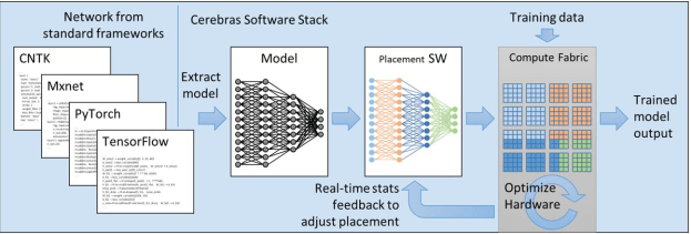
Figure 7. Cerebras Software Stack
The training uses pipelined back-propagation. The graph compiler takes the source description of the network and extracts a static graph representation of the problem and converts it into the Cerebras Linear Algebra Intermediate Representation (CLAIR). This is then converted into a “Kernel graph” and mapped to the hardware as shown in Figure 7. In their approach the entire network is mapped onto the computing fabric, so pipelining batches through has no points of congestion.
Graphcore
Graphcore is a U.K. startup started shipping their accelerator, called the Intelligence Processing Unit (IPU), in 2018 and it is now available on Azure for evaluation. Like Cerebras, the architecture is based on massively parallel processing. Each IPU contains 1,216 processing elements called tiles; a tile consists of one computing core plus 256 KiB of local memory. There is no shared memory, but the local memory is SRAM and faster than the DRAM in most CPU servers. To hide latencies, the IPU cores are multithreaded. Each core has 6 execution contexts that served in round-robin style. In terms of computational performance, each IPU is 31.1 TFlops/s in single precision.

Figure 8. Graphcore IPU
There is an inter-processor communication switch called the exchange that provides processing element data communication and multiple IPUs are connected via a fast, off-chip interface network. Citadel has published an excellent performance analysis by Jai et.al. “Dissecting the Graphcore IPU Architecture via Microbenchmarking”. They have measured “On a per-tile basis, each of the 1,216 tiles can simultaneously use 6.3 GB/s of bandwidth to transfer data to an arbitrary destination on chip. The latency of an on-chip tile-to-tile exchange is 165 nanoseconds or lower and does not degrade under load above that value.” They also measured the latencies between cores that reside on different IPU boards where several boards had to be crossed to deliver the message. This increased the latency to about 700 nanoseconds. Their report provides a very complete analysis of the data traffic performance under a variety of conditions.
Ilyes Kacher, et.al. from the European Search engine company Quant have also produced an analysis: “Graphcore C2 Card performance for image-based deep learning application: A Report”. Their interest in Graphcore was to improve performance of their image search product. In their study they considered the image analysis network ResneXt101. Inference experiments for batch sizes of 1 and 2 are 1.36 ms. Their benchmarks claim this is 40time lower latency than an Nvidia V100 GPU. They also compare performance on BERT and they measure 30% lower latency with 3 time higher throughput.
The programming model is based on Bulk Synchronous Parallelism in which computation is dived into phases, with each phase consisting of a computation step followed by a communication step and then a barrier synchronization.

Figure 9. Graphcore BSP execution (from Graphcore IPU Programmers Guide.)
https://www.graphcore.ai/products/poplar is a discussion of their stack. More significantly they have open sourced the entire software stack. They have a runtime environment called the Poplar Advanced Run Time (PopART) that can be used to load a ONNX model from python and run it on their hardware. For Tensoflow they have a separate compiler and runtime.
Graphcore hardware is now available on Azure for evaluation.
SambaNova
SambaNova is a bay area startup founded by two Stanford professors and a former executive from Sun and Oracle. They have not yet announced a product, but they have an interesting background that may indicate a very novel approach to the design of an AI accelerator.
Reconfigurable computing is an idea that has been around for since the 1960s. Field Programmable Gate Array are in common use today to configure a processor to execute a new algorithm, but these usually take 10s to 100s of milliseconds to “reprogram”. Suppose you could configure the logic elements on the chip to perform a needed transformation on a block of tensors just as that block emerges from a previous operation? The SambaNova team has looked at specialized programming languages that allow them to generate streams of high-level templated instructions such as map, reduce, shuffle and transpose that are natural elements of deep network kernels. This is clearly a talented, well-funded team and it will be interesting to see what is eventually released.
Tenstorrent
A Toronto startup called Tenstorrent has built a device called GraySkull. The chip has 120 small processing nodes, called tensix, and two toroidal mesh networks that can be extended off-chip to build larger clusters. There is no shared memory. In various articles about Tenstorrent they emphasize their approach to dealing with sparsity in large neural net models is key to high performance on big models. Like several of the other startups, their compiler translates ONNX graphs into tensix primitive operators which are mapped to the nodes. They claim 22,431 IPS on resnet 50 and 23,345 sentences/sec on BERT.
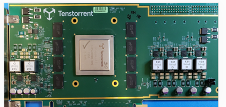
Figure 10. From Tenstorrent.
NLVDA
Finally, we include NLVDA from NVIDIA. Called a Deep Learning Accelerator, this is an open source modular architecture for building inference accelerators. There is a hardware instance called Xavier that NVIDIA has produced to support inference for autonomous transportation applications.
Compiling Neural Nets for Parallel execution.
In the remainder of this report we will look at the techniques that are used in modern compilers to optimize performance on neural network training and inference. Many of the basic techniques have been used in compilers for 50 years. These techniques evolved as CPU arithmetic and logical units became so fast that many operations were dominated by the time it took to move data from main memory through layers of faster and faster caches. Data locality was critical: if an item of data was going to be reused you needed to keep it in fast cache as long as possible.
Almost all of the operations in a neural network involve matrix and vector arithmetic. If you consider the most basic type of network layer, an n by n full connection, it is just an n by n matrix and a vector of offsets. Applying such a network to a single vector of n inputs is just a matrix-vector multiply and a vector addition. The problem with matrix-vector multiply is that the matrix elements must be fetched from memory and are used only once. On the other hand, if the computation is properly blocked so that small chunks of the array are loaded into the GPU or CPU caches, then if you have a batch of n vectors, each element of the array can be fetched once and used n times. This method of improving matrix-matrix computation is the basis of the standard library known as the Level-3 Blas developed by Jack Dongarra and others in the 1980s.
A more interesting example of how locality can be used to speed up performance in a neural network is 2-D convolutions that are used in deep learning image networks. Figure 11 below shows a 2-D convolution operating on a 6×7 image data with 3 color channels and outputs a new 6×7 array with 6 channels. Each output channel is produced by using, in this case, 3 filters of size 3×3. Each filter is applied to a channel of the input (which has been expanded with an extra border of ghost pixels). The filter moves across the input channel computing the inner product of the filter with the image at that point. The corresponding output point is the sum of the three filter inner products applied to each of the input channels.
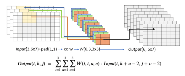
Figure 11. A 2-D convolution applied to a 3 layer, 6 by 7 image producing 6 output images.
The 6 by 3 by 9 tensor of filters, W, is the learned object and the full computation is show in the formula above (we have suppressed the bias terms to simplify the presentation). If we let Cin be the number of input channels and Cout be the number of output channels for a width by height image the full computation takes the form below. (The input is the padded (width+1) by (height+1) array, so that the pixel at position (0,0) is in location (1,1) in the array Input.)
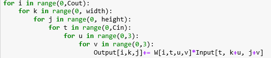
This form of the computation has extremely poor locality and it will run slowly. However, we illustrate below a sequence of program transformations that allow us to simplify this loop nest and “lower” the execution to primitives that will allow this to run up to 400 times faster.
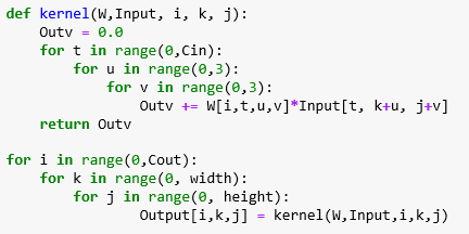
A close inspection of this nest of six loops will convince you that we can execute them in any order. In fact, the addition recurrence is only carried by the inner three loops. Consequently, we can pull out the three inner loops as a separate function that does not involve repeated writes to memory around the Output tensor. The result is shown below.
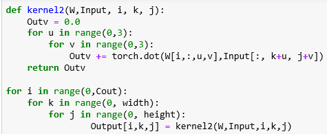
The next thing to notice is that if you move the t loop in the kernel function to the innermost position the operation is an inner product. The computation now takes the form
One final reduction can be made when we notice that the two loops in kernel2 are just a pointwise matrix product of the 3×3 filter W with the Input shifted to position (k,j). And the summation can be done with the torch.sum() function, so our function now takes the form below.
We ran these four versions of the function on two machines: an Intel core I7 and an Nvidia Jetson nano. The results are in Tables 1 and 2 below. As you can see, the performance improves substantially for each transformation. In addition, the speed up of the matrix product version over the 6 nested loop version varies from 68 to over 400 times with the greatest speedup occurring when the values of Cin are largest.
| 6 nested loops | Factored Kernel | Kernel with dotprod | Matrix product | Cin | Cout | W,H | SpeedUp |
| 2.24 seconds | 1.26 | 1.0 | 0.022 | 16 | 4 | 10,10 | 68 |
| 4.47 | 2.75 | 0.19 | 0.047 | 16 | 8 | 10,10 | 95 |
| 8.24 | 4.98 | 0.39 | 0.077 | 16 | 16 | 10,10 | 107 |
| 8.51 | 4.97 | 0.20 | 0.038 | 32 | 8 | 10,10 | 223 |
| 8.66 | 5.06 | 0.10 | 0.020 | 64 | 4 | 10,10 | 433 |
Table 1. Execution time on Intel Core i7 for the four versions of the loop with various values of Cin and Cout. The speedup is measured as the ratio of the 6 nested loop time to the time for the matrix product.
| 6 nested loops | Factored Kernel | Kernel with dotprod | Matrix product | Cin | Cout | W,H | SpeedUp |
| 47.9 seconds | 28.1 | 7.02 | 0.7 | 16 | 4 | 10,10 | 68 |
| 87.9 | 52 | 9.7 | 0.73 | 16 | 8 | 10,10 | 120 |
| 168.9 | 107 | 18.9 | 1.17 | 16 | 16 | 10,10 | 144 |
| 171 | 107.9 | 9.8 | 0.59 | 32 | 8 | 10,10 | 289 |
| 174 | 104.0 | 4.38 | 0.43 | 64 | 4 | 10,10 | 404 |
Table 2. Execution time on Nvidia Jetson Nano for the four versions of the loop with various values of Cin and Cout.
The final point to notice about this last version is the final (i,j,k) loops may all be executed in parallel. In other words, if you had a processor for each pixel on each output plane the entire operation can be run in parallel with an addition speedup factor of Cout*width*height. Of course, all of these versions are far slower than the highly optimized conv2d() library function.
The compilers we talk about below do not operate at the level of program transformation on Python loop nests. They start at a higher level, transforming ONNX-like flow graphs and eventually lowering the granularity to primitive operators and scheduling memory management and communication traffic and eventual code generation.
Deep Neural Network Compilers.
Every one of the hardware projects we described above has a companion compiler capable of mapping high level DNN frameworks like PyTorch or Tensorflow to run on their new machine. Not all of these have detailed descriptions, but some do, and some are also open source. Here is a list of a few notable efforts.
- Intel’s NGraph compiler “Adaptable Deep Learning Solutions with nGraph Compiler and ONNX” with extensive open source and documentation.
- ONNC: A Compilation Framework Connecting ONNX to Proprietary Deep Learning Accelerators. Also fully open source. It is designed to support NVDLA hardware.
- Nvidia TensorRT is an SDK for high performance inference that is built on CUDA. A TensorRT backend for ONNX is also available and open source.
- Apache TVM is an open source compiler stack for deep learning that originated with the Computer Science department of the University of Washington.
- Google MLIR, a Multi-Level IR Compiler Framework that provides tools for many types of programming language compiler challenges.
- ONNX Runtime for Transformer Inference from Microsoft has been open sourced.
- The Facebook Glow compiler “Glow: Graph lowering compiler techniques for neural networks” paper.
- The GraphCore PopART runtime was discussed in the GraphCore section above.
- Sivalingam and N. Mujkanovic of CRAY EMEA has a nice summary of these compilers in this post.
Glow translates the input from ONNX or Caffe2 into a high-level intermediate graph that is very similar to ONNX. Because they are interested in training as well as inference they next differentiate the graph to facilitate gradient decent training. This new graph contains the original and the derivative. TVM also generates a differentiable internal representation. All of the others have similar high-level internal representation. Where they differ is in the layers of transformation and lowering steps.
High Level Graph Transformations
The next step is to do optimization transformations on the graph. The nGraph compiler has a Reshape Elimination pass exploits the fact that matmul(A.t, B.t).t = matmul(B,A) and other algebraic identities to make tensor restructuring simplifications. Common subexpression elimination and constant folding are standard compiler techniques that can be applied as transformations the high-level graph. For example when compiling a model to be used for inference most of the parameters in the high level nodes, such as various tensor dimensions are known integers and expressions involve address arithmetic can be simplified.
An important part of the “lowering” process is where some of the high-level nodes are broken down into more primitive linear algebra operations. This step depends on the final target architecture: for a GPU certain transformation are appropriate and for a CPU, different choices are made. For example, with ResNet Glow has different strategies for different instances of the convolution operator depending on the size of the filter weights and these require different memory layouts. TVM, Glow and ONNC use a type of layer fusion to combine consecutive operators such as Convolution and Batchnormalization or ReLu into a single special operator.
Low Level Internal Representations
Now the graph is transformed into the Low-level internal representation. This layer is more specific about the representation of memory layout and important optimization can be made there. For example, if there are sequences of operation that must sweep across a large tensor, one can break the tensor into blocks so each block can be loaded once, and the operation sequence can be applied to the block. This is a classic locality optimization. Managing memory can involve other transformations. For example, ONNC uses layer splitting to handle memory constrains as shown in Figure 12 below.
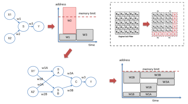
Figure 12. From Skymizer ONNC tutorial.
Quantization is an issue that several compilers address. Glow also does profile-guided quantization so that floating point networks can be converted into efficient integer-based networks. Finally, depending upon the backend architecture, code is generated from the final low-level graph.
Runtime Systems
Because the compilation system involves mapping the neural network onto hardware configurations which may have more than one processor that must communicate with each other, there must be a runtime system to handle the coordination of the execution.
Glow has a runtime system that is capable of partition networks into an acyclic graph of subgraphs and scheduled across multiple accelerators. As we have discussed previously the GraphCore PopArt runtime manages BSP-style execution across thousands of processor threads.
The Microsoft ONNX runtime focuses on CPU and CPU + GPU execution on Windows, Linux and Mac OS. For the GPU it supports CUDA, TensorRT and DirctML. It also supports IOT/Edge applications using Intel OpenVMINO, ARM and Android Neural Networks API.
Final Thoughts
The explosion of computer architecture innovation exemplified by the new systems described here is very impressive. It is reminiscent of the boom in HPC innovation in the 1990s which led to the current generation of parallel supercomputer designs. The density and scale of some of the chips are very impressive. In the 1980s we considered the impact of wafer-scale integration on parallel computing, so 40 years later, it is interesting to see it come to pass in systems like Cerebras.
There are many details of the compiler infrastructure that we covered here very superficially. We will return to this topic in the future when we have more access to details and hardware.
