Monthly Archives: January 2016

Raspberry meets Project Oxford: IoT & Judging a Book by Its Cover.

When I was (very) young I enjoyed building electronic devices from kits and from wiring diagrams I found in exciting journals like “Popular Electronics”.  Radio Shack was my friend and Heath Kits were a joy when I could afford them.   Today I marvel at the devices kids can tinker with.   They can build Arduino powered Lego robots that are lightyears beyond my childhood Lincoln Logs and Erector Sets.   And they have access to another relatively recent, world changing technology:  they have the ability to create software that brings their creations to life.  They can add sensors (accelerometers, GPS, altimeters, thermometers, gyroscopes, vibration, humidity and more) to their projects as well as actuators and motors of various types.  And these creations can live on the Internet.   Devices like the Particle (formerly Spark) Photon and Electron IoT include WiFi or cellular links so instruments can send data to the cloud.  They are programmed with the same C-like language used by the Arduino.   Photon devices are extremely small and very inexpensive so they can be deployed in very large numbers.

Indeed, these devices are the atomic particles of the Internet of Things (IoT).  They are being turned into modestly built home safety sensors as well as sophisticated instruments that control highly sensitive scientific experiments.   They will be the tools city planners will use to understand our complex urban environments.   For example, the Array of Things project at the University of Chicago and Argonne Labs is deploying an amazing small sensor pack on that will sit on light polls throughout the city.   (Check out this video.)  Charlie Catlett and Pete Beckman are leading the AoT project.  In discussions with Charlie he told me that he has built a full array of sensors in his home to monitor various devices.   He also pointed me to the Mathworks Thingspeak product which provides a lovely Matlab-based cloud platform for integrating and analyzing the streams of data from your instruments.

In a previous post I described ways in which event data could be streamed to the cloud and I will return to that topic again in the future.   In this article I wanted to look at what could be done with a small device with a video camera when it was combined with analysis on the Cloud.  I chose the Raspberry Pi2 and the cloud services from the new Microsoft Research project Oxford services.

Phone Apps and Project Oxford

While the instruments described above will eventually dominate the Internet of Things, the billions of smart phones out there today give us a pretty good idea of the challenge of managing data from sensors.   Almost every truly useful “App” on a smart phone interacts services in the cloud in order to function properly.    And each of these apps does part of its computation locally and part takes place remotely.   Cortana and Siri can do the speech to text translation by invoking a speech model on the phone but answering the query involves another set of models running in the cloud.    For any interesting computational task, including the tasks assigned to the Array of Things sensors, some computation must be done locally and some must be remote.   In some cases, the local computation is needed to reduce the amount of time spent communicating with the back end services and in other cases, for example for privacy reasons, not all locally collected information should be transmitted to the cloud.  (What happens to my phone in Vegas, should stay in Vegas.)  Indeed, according to Catlett and Beckman, protecting privacy is a prime directive of the Array of Things project.

Companies like Amazon, Google, IBM, Microsoft and Salesforce have been working hard to roll out data analytics services hosted on their cloud platforms.   More recently these and other companies have been providing machine learning services in the cloud.   I have already talked about AzureML, a tool that allows you to build very powerful analysis tools, but for people who want to build smart apps there are now some very specialized services that do not require them to be ML domain experts.  A good example is IBMs Watson Services that is a result of IBM’s work on bringing their great Jeopardy playing capability to a much broader class of applications.  Watson has a great collection of language and speech analysis and translation services.   In addition, it has an impressive collection of image analysis tools.

Project Oxford is another interesting collection of cloud services that cover various topics in computer vision, speech and language.  In the area of speech, they provide the APIs needed for speech to text and text to speech.  We are all familiar with the great strides taken in speech recognition with Siri, Cortana, Echo and others.   With these APIs one can build apps for IOS, Windows and Android that use speech recognition or speech generation.   The language tools include spell checkers, a nifty language understanding tool that you can train to recognize intent and action from utterances such as commands like “set an alarm for 1:00 pm.”  The computer vision capabilities include scene analysis, face recognition, and optical character recognition (OCR).  These are the services I will explore below.

Raspberry Pi2 and the OpenCV computer vision package.

The Raspberry Pi 2 is a very simple, credit card sized, $35 single board computer with a very versatile collection of interfaces. It has a Broadcom VideoCore GPU and a quad-core ARMv7 processor and 1 GB of memory.  For a few extra dollars you can attach a five-megapixel camera.  (In other words, it is almost as powerful as a cellphone.) The Pi2 device can run Windows 10 IoT Core or a distribution of Linux.  I installed Linux because it was dead easy.   To experiment with the camera, I needed the OpenCV computer vision tools.  Fortunately, Adrian Rosebrock has documented the complete installation process in remarkable detail.  (His book also provides many useful coding example that I used to build my experiments.)

Object Tracking

One of the most obvious sensing challenges one can tackle with a small Interconnected device with a camera is object tracking.   With OpenCV there are some very sophisticated ways to do this, but for some tasks it is trivial.   Outside my window there is a small harbor and I decided to track the movements of the boats.   This was easy because they are all pleasure boats so the vast majority of them are white.  By filtering the image to bring out white objects on a black background the OpenCV functions “findContours” and “minAreaRect” it requires only a few lines of code to draw bounding boxes around suspected boats. (Full source code for the examples here are in Github.) With the Pi device and camera sitting near the window.  I was able to capture the scene below in Figure 1.  Note that it took some scene specific editing.  Specifically, it was necessary to ignore contours that were in the sky.   As can be seen some objects that were not boats were also selected.    The next step is to filter based on the motion of the rectangles.  Those are the rectangles worth tracking. Unfortunately, being winter these pleasure craft haven’t moved for a while, so I don’t have a video to show you.

boats2-capture

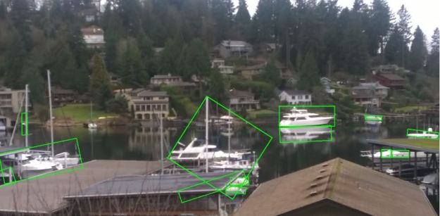
Figure 1.   Using OpenCV to find boats in a harbor

Face Recognition

By face recognition we mean identifying those elements in a picture that are human faces. This is a far lower bar than face identification (who is that person?), but it is still an interesting problem and potentially very useful.  For example, this could be used to approximate the number of people in a scene if you know what fraction of them are facing the camera.   Such an approximation may be of value if you only wanted to know the density of pedestrian traffic.  You could avoid privacy concerns because you would not need to save the captured images to non-volatile storage. It is possible to use OpenCV alone to recognize faces in a picture and never send the image outside the device.

If you do want to know more information about a group of people project Oxford can do much better.  Given an image of a group it can identify the faces looking in the general direction of the camera and for each face it can give a number of interesting features such as gender, estimated age and even a “smile” index.   This information may be of interest to a business, such as a movie theater owner who wants to know the gender makeup and average age of the of the patrons.  It could even tell by counting smiles if they enjoyed the movie.    I used project Oxford to do an analysis of two photos.   The first is our class of amazing students and staff from the 2014 MSR summer school in Moscow.   The vision service also returned a rectangle enclosing each face.   I use OpenCV to draw the rectangle with a pink border for the males and green for females if they were smiling.   If they were not smiling, they got a black rectangle.  As can be seen, the reporting was very accurate for this staged group photo.

yandex-face-out

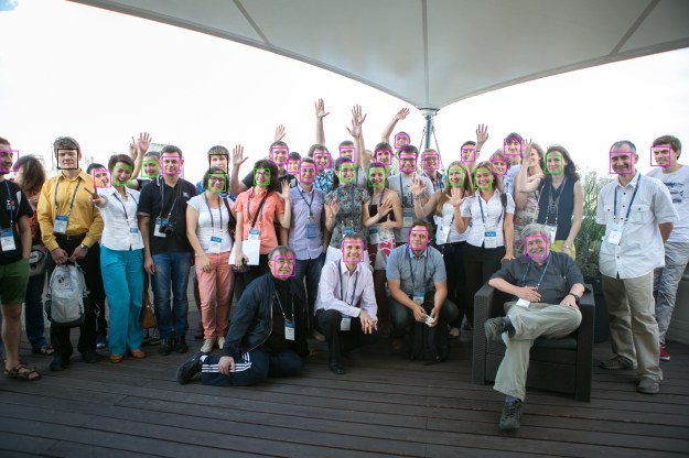
Figure 2.   Project Oxford Face Recognition of MSR Summer School 2014 group photo taken at Yandex headquarters Moscow.  Pink = male, green = female, black = no smile

The system also allowed us to compute estimated average age: approximately 21 for females, 24 for males.  (Some “senior” professors in the photo skewed the average for males.).   Figure 3 below shows the result for a stock street scene.  Very few smiling faces, but that is not a surprise.   It also illustrates that the system is not very good at faces in partial or full profile.

sidewalk-crowd-face-out

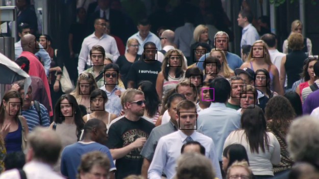
Figure 3.   Many faces missing in this crowd, but one is smiling.

Text Recognition

Optical Character Recognition (OCR) has been around for use in document scanners for a long time but it is much harder to read text when it is embedded in a photo with other objects around it.    For example, programing the Pi using a call to oxford OCR and pointing the camera at the image in Figure 4 produced the output in the superimposed rectangle (superimposition done with PowerPoint … not OpenCV).

oxford-text-out-final

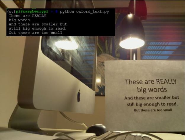
Figure 4.   Oxford OCR test from Pi with command line output in black rectangle.

As can be seen, this was an easy case and it made only one error.     However, it is not hard to push the OCR system beyond its limits based on distance, lighting and the angle of the image.

To demonstrate the power of doing some computation on the local device and some of it remotely in the cloud, we can take an scene that is too hard for oxford to understand directly and so some preprocessing with OpenCV.   In Figure 5 we have taken a scene with the same piece of paper with text and placed it far from the camera and at a funny angle.   This yielded no result with Oxford OCR directly.   But in this case we used the same filtering technique used in the boat tracking experiment and located the rectangle containing the paper.  Using another OpenCV transformation we transformed that rectangle into a 500 by 300 image with the rotation removed (as shown in the insert).   We sent that transformed image to Oxford and got a partial result (shown in the black rectangle).

oxford-text-out-with-opencv

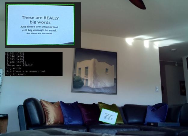
Figure 5.  Transformed image and output showing the coordinates of the bounding rectangle and output from Oxford OCR.   The green outline in the picture was inserted by OpenCV drawing functions using the bounding rectangle.

This experiment is obviously contrived.  How often do you want to read text at a distance printed on a white rectangle?  Let’s look at one final example below.

Judging a Book by Its Cover

An amusing App that may be able to use the Oxford OCR would be to use it to find information about a book based on an image of the cover.   Of course, this is not a new idea.  Amazon has an app called “Flow” from their A9 Innovations subsidiary.  More on that later.    What  I did was to integrate Oxford OCR with a call to Bing.    It works as follows.  The Pi is shown the image of a book,  the OCR app looks for text on the image like the title or author.   Then that returned string is sent to Bing via a web service call.   The top five results are then put into an HTML document along with the image and served up by a tiny webserver on the PI.   The first results are shown below.

bing-reader-out1

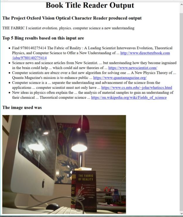
Figure 6.   Output of the book cover reader app webserver on the PI.  The first result is correct.

The interesting thing about this is that Bing (and I am sure Google as well) is powerful enough to take partial results from the OCR read and get the right book on the top hit.  The correct text is

The Fabric of Reality.   A leading scientist interweaves evolution, theoretical Physics and computer science to offer a new understanding of reality.”  (font changes are reproduced as shown on the book cover)

What the OCR systems was able to see was “THE FABRIC I scientist evolution, physics. Computer science a new understanding.”   The author’s name is occluded by a keyboard cable.

Unfortunately, the reliability at a distance was not great.  I next decided to try to enhance the image using the technique used in the “text on white rectangle” as illustrated in Figure 5.    Of course this needed a white book, so it is not really practical.  However, the results did improve the accuracy (for white books).   An example that the OCR-only version failed to recognize but that worked using the OpenCV enhanced version is shown in Figure 7.

black_swawn

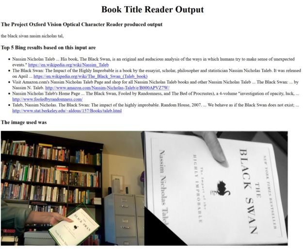
Figure 7.   Using OpenCV with Oxford and Bing.

As can be seen the OCR saw “the black sivan nassim aicholas tal”, which is not very accurate. Even with the lower right corner of the book out of the image I would have expected it to do a bit better.   But Bing was easily able to figure it out.

I downloaded the Flow app and installed it on a little Android tablet.   It works very well up close but it could not handle the distance shots illustrated above.   Of course this is not a proper scientific comparison.    Furthermore, I have only illustrated a few trivial features of OpenCV and I have not touch the state-of-the-art object recognition work.  Current object recognition systems based on deep learning are amazingly accurate.  For example, MSR’s Project Adam was used to identify thousands of different types of object in images (including hundreds of breeds of dogs).   I expect that Amazon has the images of tens of thousands of book covers.   A great way to do the app above would be to train a deep network to recognize those objects in an image.  I suspect that Flow may have done something like this.

Final Thoughts

The examples above are all trivial in scope, but they are intended to illustrate what one can do with a very simple little device, a few weeks of programming and access to tools like Project Oxford.   We started with a look at IoT technologies and moved on to simple “apps” that use computer vision.   This leads us to think about the topic of augmented reality where our devices are able to tell us about everything and everyone around us.   The “everyone” part of this is where we have the most difficulty.   I once worked on a project called the “intelligent memory assistant”.   Inspired by a comment from Dave Patterson, the app would use a camera and the cloud to fill in the gaps in your memory so that when you met a person but could not remember their name or where they were from.  It would whisper into your ear and tell you “This is X and you knew him in 1990 …. “.  It is now possible to build this, but the privacy issues raise too many problems.   It is sometime referred to as the “creepy factor”. For example, people don’t always want to be “tagged” in a photo on Facebook.   On the other hand uses like identifying lost children or amnesiacs are not bad. And non-personal components of augmented reality are coming fast and will be here to stay.

PS Code for these examples is now in this github repo

An Encounter with Google’s TensorFlow

NOTE: This is a revised version of this blog that reflects much better ways to do some of the tensor algebra in the first example below.

Google has recently released some very interesting new tools to the open source community.   First came Kubernetes, their container microservice framework, and that was followed by two new programming systems based on dataflow concepts.   Dataflow is a very old idea that first appeared in the computer architecture community in the 1970 and 80s.   Dataflow was created as an alternative to the classical von-Neumann computer design.  It was hoped that it would have a performance advantage because it would exploit much greater levels of parallelism than thought possible with classical computers[1].  In dataflow systems computation can be visualized as a directed graph where the vertices of the graph are operators and data “flows” through the system along the edges of the graph.  As soon as data is available on all the input edges of an operator node the operation is carried out and new data is put on the output edges of the node.  While only a few actual data flow computers were built, the concept has been fundamental to distributed and parallel computing for a long time.  It shows up in applications like complex event processing, stream analytics and systems like the Microsoft AzureML programming model I described earlier.

Google’s newly released Cloud Dataflow is a programming system for scalable stream and batch computing.  I will return to Cloud Dataflow in another post, but for now, I will focus on the other dataflow system they released.  Called TensorFlow, it is a programming system designed to help researchers build deep neural networks[2] and it appears to be unrelated to Cloud Dataflow.  All the documentation and downloadable code for TensorFlow are on-line.  TensorFlow is also similar to Microsoft Research’s Computational Network Toolkit (CNTK) in several ways that I will describe later.

TensorFlow is designed allow the programmer to easily “script” a dataflow computation where the basic units of computing are very large multi-dimensional arrays.   The scripts are written in Python or C++ and it works very well with IPython/jupyter notebooks.   In the following pages I will give a very light introduction to TensorFlow programming and illustrate it by building a bare-bones k-means clustering algorithm.   I will also briefly describe one of their examples of a convolutional neural network.

TensorFlow can be installed and run on your laptop, but as we shall show below, it really shines on bigger more powerful hardware.  An interesting thing happened in the recent evolution of deep neural networks.   The most impressive early work on really large deep neural network was done on large cloud-scale clusters.  However, the type of parallelism needed for doing deep network computation was really very large array math, which is really better suited to execution on a GPU.  Or a bunch of GPUs on a massive memory machine or a cluster of massive memory machines with a bunch of GPUs each.  For example, the Microsoft CNTK has achieved some remarkable results on 8 GPU systems and it will soon be available on the Azure GPU Lab. (I also suspect that supercomputers such as the SDSC Comet with large memory, multi-GPU, multi-core nodes would be ideal.)

TensorFlow: a shallow introduction.

There is a really nice white paper by the folks at Google Research with far more details about the TensorFlow system architecture than I give here.  What follows is a shallow introduction and an experiment.

There are two main concepts in TensorFlow.   The first is the idea of computing on objects that are very large multi-dimensional arrays called tensors.   The second is the fact that the computation you build with tensors are compiled into graphs that are executed in a “dataflow” style.   We need to unpack both of these concepts.

Tensors

Let’s start with tensors.  First, these are not your great-great grandfather’s tensors.   Those tensors were introduced by Carl Friedrich Gauss for differential geometry where they were needed to provide metrics that could be used to describe things like the curvature of surfaces.  Einstein “popularized” tensors in his general theory of relativity.  Those tensors have a very formal algebra of covariant and contravariant forms. Fortunately, we don’t have to go there to understand the use of tensors in TensorFlow’s machine learning applications.   In fact, if you understand Numpy arrays you are off to a good start and Numpy arrays are just really efficient multidimensional arrays.   TensorFlow can be programmed in Python or C++ and I will use the Python binding in the discussion below

In TensorFlow tensors are created and stored in container objects that are one of three types: variables, placeholders and constants.   Let’s start with constants.  As the name implies constant tensors are initialized once and never changed.   Here are two different ways to create constant arrays that we will use in an example below.  One is a tensor of size Nx2 filled with zeros and the other is a tensor of the same shape filled with the value 1.

import numpy as np
import tensorflow as tf
N = 10000
X = np.zeros(shape=(N,2))
Xv = tf.constant(X, name="points")
dones = tf.fill([N,2], np.float64(1.))

We have used a Numpy array of values to create the TensorFlow constant. Notice that we have given our tensor a “name”. Naming tensors is optional but it comes in very handy when debugging.
Variables are holders of multidimensional arrays that persist across sessions and may be modified and even saved to disk. The concept of a “session” is important in TensorFlow. You can think of it as a context where actual TensorFlow calculations take place. The first calculation involving a variable is to load it with initial values. For example, let’s create a 2 by 3 tensor that, when initialized contains the constant 1.0 in every element. Then let’s convert that back to a Numpy array and print it. To do that we need a session and we will call the variable initializer in that session. When working in the IPython notebook it is easiest to use an “InteractiveSession” so that we can easily edit and redo computations.

sess = tf.InteractiveSession()
myarray = tf.Variable(tf.constant(1.0, shape = [2,3]))
init =tf.initialize_all_variables()
sess.run(init)
mynumpy =myarray.eval()
print(mynumpy)
[[ 1.  1.  1.]
 [ 1.  1.  1.]]

As shown above, the standard way to initialize variables is to initialize them all at once. The process of converting a tensor back to a Numpy array requires evaluating the tensor with the “eval” method. As we shall see this is an important operator that we will describe in more detail below.

The final tensor container is a “placeholder”.   Creating a placeholder object only requires specifying a type and some information about its shape.   We don’t initialize a placeholder like a variable because it’s initial values will be provided later in an eval()-like operation.  Here is a placeholder we will use later.

x = tf.placeholder(tf.float32, [None, 784], name="x")

Notice that in this case the placeholder x is two dimensional but the first dimension is left unbound.  This allows us to supply it with a value that is any number of rows of vectors of length 784.   As we shall see, this turns out to be very handy for training neural nets.

Dataflow

The real magic of TensorFlow is in the dataflow execution of computations.   A critical idea behind TensorFlow is to keep the slow world of Python away from the fast world of parallel tensor algebra as much as possible.  Python is used only to describe the dataflow graph of the computation.   TensorFlow has a large library of very useful tensor operators.   Let’s describe a computation we will use in the k-means example.   Suppose we have 8 points in the plane in a vector called Xv and 4 special points in an array called kPoints.   I would like to label each of the 8 points with the index of the special point nearest to it.   This should give me 4 clusters of points.   I now want to find the centroid of each of these clusters.  Assume we have a tensor called “blocked” where row i gives the distance from each of our 8 points to the ith special point.  For example, if “blocked” is as shown below then what we are looking for is the index of the smallest element in each column.tensor-table

To find the centroids I use this min index vector to select the elements of Xv in each cluster. We just add them up to and divide by the number of points in that cluster.    The TensorFlow code to do this is shown below.  TensorFlow has a large and handy library of tensor operators many of which are similar to Numpy counterparts.   For example, argmin computes the index of the smallest element in an array given the dimension over which to search.   Unsorted_segment_sum will compute a sum using another vector to define the segments.   The min index vector nicely partitions the Xv vector into the appropriate “segments” for the unsorted_segment_sum to work.  The same unsorted_segment_sum operator can be used to count the number of elements in each cluster by adding up 1s.

mins = tf.argmin(blocked, 0, name="mins")
sums = tf.unsorted_segment_sum(Xv, mins, 4)
totals = tf.unsorted_segment_sum(dones, mins, 4, name="sums")
centroids = tf.div(sums, totals, name = "newcents")

The key idea is this.  When this python code is executed it builds a data flow graph with three inputs (blocked, Xv, dones) and outputs a tensor called centroids as shown below[3].[4]

The computation does not start until we attempt to evaluate the result with a call to centroids.eval(). This sort of lazy evaluation means that we can string together as many tensor operators as needed that will all be executed outside the Python REPL.

tensor-graph1

Figure 1.  Computational flow graph

TensorFlow has a very sophisticated implementation.  The computing environment upon which it is running is a collection of computational devices.  These devices may be cpu cores, GPUs or other processing engines.   The TensorFlow compilation and runtime system maps subgraphs of the flow graph to these devises and manages the communication of tensor values between the devices.  The communication may be through shared memory buffers or send-receive message pairs inserted in the graph at strategically located points.   Just as the dataflow computer architects learned, dataflow by itself is not always efficient.  Sometimes control flow is needed to simplify execution.  The TensorFlow system also inserts needed control flow edges as part of its optimizations.   As was noted above, this dataflow style of computation is also at the heart of CNTK.   Another very important property of these dataflow graphs is that it is relatively easy to automatically compute derivatives by using the chain-rule working backwards through the graph.   This makes it possible to automate the construction of gradients that are important for finding optimal parameters for learning algorithms.   I won’t get into this here but it is very important.

A TensorFlow K-means clustering algorithm

With the kernel above we now have the basis for a simple k-means clustering algorithm shown in the code below.  Our initial centroid array is a 4 by 2 Numpy array we shall call kPoints.   What is missing is the construction of the distance array blocked.   Xv holds all the N points as a constant tensor.   My original version of this program used python code to construct blocked.  But there is an excellent improvement on computation of “mins” published in GitHub by Shawn Simister at.  Shawn’s version is better documented and about 20% faster when N is in the millions.  Simister’s computation does not need my blocked array and instead expands the Xv and centroids vector and used a reduction to get the distances.  Very nice (This is the revision to the blog post that I referred to above.)

N = 10000000
k = 4
#X is a numpy array initialized with N (x,y) points in the plane
Xv = tf.constant(X, name="points")
kPoints = [[2., 1.], [0., 2.], [-1., 0], [0, -1.]]
dones = tf.fill([N,2], np.float64(1.))

centroids = tf.Variable(kPoints, name="centroids")
oldcents = tf.Variable(kPoints)
initvals = tf.constant(kPoints, tf.float64)

for i in range(20):
    oldcents = centroids
    #This is the Simister mins computation
    expanded_vectors = tf.expand_dims(Xv, 0)
    expanded_centroids = tf.expand_dims(centroids, 1)
    distances = tf.reduce_sum( tf.square(
               tf.sub(expanded_vectors, expanded_centroids)), 2)
    mins = tf.argmin(distances, 0)
    #compute the new centroids as the mean of the points nearest
    sums = tf.unsorted_segment_sum(Xv, mins, k)
    totals = tf.unsorted_segment_sum(dones, mins, k, name="sums")
    centroids = tf.div(sums, totals, name = "newcents")
    #compute the distance the centroids have moved sense the last iteration
    dist = centroids-oldcents
    sqdist = tf.reduce_mean(dist*dist, name="accuracy")
    print np.sqrt(sqdist.eval())
    kPoints = centroids.eval()

However, this version is still very inefficient.  Notice that we construct a new execution graph for each iteration.   A better solution is to pull the graph construction out of the loop and construct it once and reuse it.   This is nicely illustrated in Simister’s version of K-means illustrated on his Github site.

It is worth asking how fast Tensor flow is compared with a standard Numpy version of the same algorithm. Unfortunately, I do not have a big machine with fancy GPUs, but I do have a virtual machine in the cloud with 16 processors. I wrote a version using Numpy and executed them both from an IPython notebook. The speed-up results are in Figure 2. Comparing these we see that simple Python Numpy is faster than TensorFlow for values of N less than about 20,000. But for very large N we see that TensorFlow can make excellent use of the extra cores available and exploits the parallelism in the tensor operators very well.

kmeans-speed

Figure 2. speed-up of TensorFlow on 16 cores over a simple Numpy implementation. The axis is log10(N)

I have placed the source for this notebook in Github. Also an improved version based on Simister’s formulation can be found there.

TensorFlow also has a very interesting web tool call TensorBoard that lets you look at various aspects of the logs of your execution. One of the more interesting TensorBoard displays is the dataflow graph for your computation. Figure 3 below shows the display generated for the k-means computational graph.

tensorboard

Figure 3.   TensorBoard graph displace of the k-means algorithm.

As previously mentioned this is far more complex than my diagram in Figure 1.   Without magnification this is almost impossible to read.  Figure 4 contains a close-up of the top of the graph where the variable newcents is created.   Because this is an iteration the dataflow actually contains multiple instances and by clicking on the bubble for the variable it will show you details as shown in the close-up.

tensorboard3

Figure 4.   A close-up of part of the graph showing expanded view of the multiple instances of the computation of the variable newcents.

A brief look at a neural network example

The k-means example above is really just an exercise in tensor gymnastics. TensorFlow is really about building and training neural networks.   The TensorFlow documents have a number of great example, but to give you the basic idea I’ll give you a brief look at their convolutional deep net for the MNIST handwritten digit example.   I’ll try to keep this short because I will not be adding much new here. The example is the well-known “hello world” world of machine learning image recognition.   The setup is as follows.   You have thousands of 28 by 28 black and white images of hand written digits and the job of the system you build is to identify each.   The TensorFlow example uses a two-layer convolutional neural net followed by a large, densely connected layer and a readout layer.

If you are not familiar with convolutional neural nets, here is the basic idea.   Images are strings of bits but they also have a lot of local 2d structure such as edges or holes or other patterns.  What we are going to do is look at 5×5 windows to try to “find” these patterns.  To do this we will train the system to build a 5×5 template W array (and a scalar offset b) that will reduce each 5×5 window to a point in a new array conv by the formula

conv-formula

(the image is padded near the boundary points in the formula above so none of the indices are out of bounds)

We next modify the conv array by applying the “ReLU” function max(0,x) to each x in the conv array so it has no negative values.   The final step is to do “max pooling”.  This step simply computes the maximum value in a 2×2 block and assigns it to a smaller 14×14 array.   The most interesting part of the convolutional network is the fact that we do not use one 5×5 template but 32 of them in parallel producing 32 14×14 result “images” as illustrated in Figure 5 below.convolutional

Figure 5.   The first layer convolutional network.

When the network is fully trained each of the 32 5×5 templates in W is somehow different and each selects for a different set of features in the original image. One can think of the resulting stack of 32 14×14 arrays (called h_pool1) as a type of transform of the original image much as a Fourier transform can separate a signal in space and time and transform it into frequency space. This is not what is going on here but I find the analogy helpful.
We next apply a second convolutional layer to the h_pool1 tensor but this time we apply 64 sets of 5×5 filters to each the 32 h_pool1 layers (and adding up the results) to give us 64 new 14×14 arrays which we reduce with max pooling to 64 7×7 arrays called h_pool2.

Rather than provide the whole code, which is in the TensorFlow tutorial,  I will skip the training step and show you how you can load the variables from a previous training session and use them to make predictions from the test set. .   (The code below is modified versions of the Google code found at GitHub and subject to their Apache copyright License.)

Let’s start by creating some placeholders and variables.  We start with a few functions to initialize weights.   Next we create a placeholder for our image variable x which is assumed to be a list of 28×28=784 floating point vectors.  As described above, we don’t know how long this list is in advance. We also define all the weights and biases described above.

def weight_variable(shape, names):
  initial = tf.truncated_normal(shape, stddev=0.1)
  return tf.Variable(initial, name=names)

def bias_variable(shape, names):
  initial = tf.constant(0.1, shape=shape)
  return tf.Variable(initial, name=names)

x = tf.placeholder(tf.float32, [None, 784], name="x")

sess = tf.InteractiveSession()

W_conv1 = weight_variable([5, 5, 1, 32], "wconv")
b_conv1 = bias_variable([32], "bconv")
W_conv2 = weight_variable([5, 5, 32, 64], "wconv2")
b_conv2 = bias_variable([64], "bconv2")
W_fc1 = weight_variable([7 * 7 * 64, 1024], "wfc1")
b_fc1 = bias_variable([1024], "bfcl")
W_fc2 = weight_variable([1024, 10], "wfc2")
b_fc2 = bias_variable([10], "bfc2")

Next we will do the initialization by loading all the weight and bias variable that were saved in the training step. We have saved these values using TensorFlow’s save state method previously in a temp file.

saver = tf.train.Saver()
init =tf.initialize_all_variables()
sess.run(init)
saver.restore(sess, "/tmp/model.ckpt")

We can now construct our deep neural network with a few lines of code. We start with two functions to give us a bit of shorthand to define the 2D convolution and max_pooling operators. We first reshape the image vectors into the image array shape that is needed. The construction of the flow graph is now straight forward. The final result is the tensor we have called y_conv.

def conv2d(x, W):
  return tf.nn.conv2d(x, W, strides=[1, 1, 1, 1], padding='SAME')

def max_pool_2x2(x):
  return tf.nn.max_pool(x, ksize=[1, 2, 2, 1],
                        strides=[1, 2, 2, 1], padding='SAME')

#first convolutional layer
x_image = tf.reshape(x, [-1,28,28,1])
h_conv1 = tf.nn.relu(conv2d(x_image, W_conv1) + b_conv1)
h_pool1 = max_pool_2x2(h_conv1)
#second convolutional layer
h_conv2 = tf.nn.relu(conv2d(h_pool1, W_conv2) + b_conv2)
h_pool2 = max_pool_2x2(h_conv2)
#final layer
h_pool2_flat = tf.reshape(h_pool2, [-1, 7*7*64])
h_fc1 = tf.nn.relu(tf.matmul(h_pool2_flat, W_fc1) + b_fc1)
y_conv=tf.nn.softmax(tf.matmul(h_fc1, W_fc2) + b_fc2)

Notice that we have not evaluated the flow graph even though we have the values for all of the weight and bias variables already loaded. We need a value for our placeholder x. Suppose tim is an image from the test set. To see if our trained network can recognize it all we need to do is supply it to the network and evaluate. To supply the value to the network we use the eval() function with a special “feed_dict” dictionary argument. This just lists the name of the placeholder and the value you wish to give it.

tim.shape = ((1,28*28))
y = y_conv.eval(feed_dict={x: tim})
label = np.argmax(y)
print(label)

You can read the TensorFlow tutorial to learn about the network training step.   They use a special function that does the stochastic backpropagation that makes it all look very simple.

How does this thing work?

Developing an intuition for how the convolutional neural network actually works is a real challenge.  The fact that it works at all is amazing.  The convolutional steps provide averaging to help create a bit of location and scale invariance, but there is more going on here.   Note that given a 28*28 image the output of the second convolutional step is 64 7×7 array that represent feature activations generated by the weight templates.   It is tempting to look at these as images to see if one can detect anything.  Obviously the last fully connected layer can do a great job with these.   But it is easy to see what they look like.   If we apply h_pool2.eval(feed_dict={x: image}) we can look at the result as a set of 64 images.  Figure 6 does just that.  I picked two random 9 images, two 0s, two 7s and three 6s.   Each column in the figure represents depicts the first 9 of the 64 images generated by each.    If you stare at this long enough you can see some patterns there.  (Such as the diagonals in the 7s and the cup shape of the 4s.) But very little else.   On the other hand, taken together each (complete) column is a sufficient enough signature for the last layer of the network to identify the figure with over 99% accuracy.   That is impressive.

conv_digits.JPG

Figure 6.  Images of h_pool2 given various images of handwritten digits.

I have put the code to generate these images on Github along with the code to train the network and save the learned weights.  In both cases these are ipython notebooks.

A much better way to represent the data learned in the convolutional networks is to “de-convolve” the images back to the pixel layers.  In Visualizing and Understanding Convolutional Networks by Matthew Zeiler and Rob Fergus do this and the results are fascinating.

Final Notes

I intended this note to be a gentle introduction to the programming style of TensorFlow and not an introduction to deep neural networks, but I confess I got carried away towards the end.   I will follow up this post with another that look at recurrent networks and text processing provided I can think of something original to say that is not already in their tutorial.

I should also note that the construction of the deep network is, in some ways, similar to Theano, the other great Python package for building deep networks.  I have not looked at how Theano scales or how well it can be used for tasks beyond deep neural networks, so don’t take this blog as an endorsement of TensorFlow over Theano or Torch.

On a final note I must say that there is another interesting approach to image recognition problem.  Antonio Criminisi has led a team that has developed Deep Neural Decision Forests that combine ideas from decision forests and CNNs.

[1] This was before the explosion of massively parallel systems based on microprocessors changed the high-end computing world.

[2] If you are new to neural networks and deep learning, you may want to look at Michael Nielsen’s excellent new on-line book. There are many books that introduce deep neural networks, but Nielsen’s mathematical treatment is very clear and approachable.

[3] This is not a picture of the actual graph that is generated.   We will use another tool to visualize that later in this note.

[4] The observant reader will note that we have a possible divide by zero here if one of the special points is a serious outlier.   As I said, this is a bare-bones implementation.