Category Archives: python

Parallel Programming in the Cloud with Python Dask

I am always looking for better ways to write parallel programs.  In chapter 7 of our book “Cloud Computing for Science and Engineering” we looked at various scalable parallel programming models that are used in the cloud.   We broke these down into five models: (1) HPC-style “Single Program Multiple Data” (SPMD) in which a single program communicates data with copies of itself running in parallel across a cluster of machines, (2) many task parallelism that uses many nearly identical workers processing independent data sets, (3) map-reduce and bulk synchronous parallelism in which computation is applied in parallel to parts of a data set and intermediate results of a final solution are shared at well defined, synchronization points,  (4) graph dataflow transforms a task workflow graph into sets of parallel operators communicating according to the workflow data dependencies and (5) agents and microservices  in which a set of small stateless services process incoming data messages and generate messages for other microservices to consume.  While some applications that run in the cloud are very similar to the batch style of HPC workloads, parallel computing in the cloud is often driven by different classes application requirements.  More specifically, many cloud applications require massive parallelism to respond external events in real time.  This includes thousands of users that are using apps that are back-ended by cloud compute and data.   It also includes applications that are analyzing streams of data from remote sensors and other instruments.   Rather than running in batch-mode with a start and end, these applications tend to run continuously.

A second class of workload is interactive data analysis.   In these cases, a user is exploring a large collection of cloud resident data.   The parallelism is required because the size of the data: it is too big to download and if you could the analysis would be too slow for interactive use.

We have powerful programming tools that can be used for each of the parallel computing models described above but we don’t have a single programming tool that support them all.   In our book we have used Python to illustrate many of the features and services available in the commercial clouds.  We have taken this approach because Python and Jupyter are so widely used in the science and data analytics community.  In 2014 the folks at Continuum (now just called Anaconda, Inc) and a several others released a Python tool called Dask which supports a form of parallelism similar to at least three of the five models described above.  The design objective for Dask is really to support parallel data analytics and exploration on data that was too big to keep in memory.   Dask was not on our radar when we wrote the drafts for our book,  but it certainly worth discussing now.

Dask in Action

This is not intended as a full Dask tutorial.   The best tutorial material is the on-line YouTube videos of talks by Mathew Rocklin from Anaconda.   The official  tutorials from Anaconda are also available.  In the examples we will discuss here we used three different Dask deployments.  The most trivial (and the most reliable) deployment was a laptop installation.  This worked on a Windows 10 PC and a Mac without problem.  As Dask is installed with the most recent release of Anaconda, simply update your Anaconda deployment and bring up a Jupyter notebook and “import dask”.    We also used the same deployment on a massive Ubuntu linux VM on a 48 core server on AWS.  Finally, we deployed Dask on Kubernetes clusters on Azure and AWS.

Our goal here is to illustrate how we can use Dask to illustrate several of the cloud programming models described above.    We begin with many task parallelism, then explore bulk synchronous and a version of graph parallelism and finally computing on streams.  We say a few words about SPMD computing at the end, but the role Dask plays there is very limited.

Many Task Parallelism and Distributed Parallel Data Structures

Data parallel computing is an old important concept in parallel computing.  It describes a programming style where a single operation is applied to collections of data as a single parallel step. A number of important computer architectures supported data parallelism by providing machine instructions that can be applied to entire vectors or arrays of data in parallel.  Called Single instruction, multiple data (SIMD) computers, these machines were the first supercomputers and included the Illiac IV and the early Cray vector machines.  And the idea lives on as the core functionality of modern GPUs.   In the case of clusters computers without a single instruction stream we traditionally get data parallelism by distributed data structures over the memories of each node in the cluster and then coordinating the application of the operation in a thread on each node in parallel.   This is an old idea and it is central to Hadoop, Spark and many other parallel data analysis tools.   Python already has a good numerical array library called numpy, but it only supports sequential operations for array in the memory of a single node.

Dask Concepts

Dask computations are carried out in two phases.   In the first phase the computation is rendered into a graph where the nodes are actual computations and the arcs represent data movements.   In the second phase the graph is scheduled to run on a set of resources.  This is illustrated below.  We will return to the details in this picture later.

dask-workflow

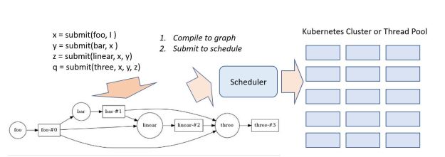
Figure 1.  Basic Dask operations: compile graph and then schedule on cluster

There are three different sets of “resources” that can be used.   One is a set of threads on the host machine.   Another is a set of process and the third is a cluster of machines.   In the case of threads and local processes the scheduling is done by the “Single machine scheduler”.   In the case of a cluster it called the distributed cluster.  Each scheduler consumes a task graph and executes it on the corresponding host or cluster.   In our experiments we used a 48 core VM on AWS for the single machine scheduler. In the cluster case the preferred host is a set of containers managed by Kubernetes.   We deployed two Kubernetes clusters:  a three node cluster on Azure and a 6 node cluster on AWS.

Dask Arrays, Frames and Bags

Python programmers are used to numpy arrays, so Dask takes the approach to distributing arrays by maintaining as much of the semantics of numpy as possible.  To illustrate this idea consider the following numpy computation that creates a random 4 by 4 array, then zeros out all elements lest than 0.5 and computes the sum of the array with it’s transpose.

x = np.random.random((4,4))
x[x<0.5] = 0
y = x+x.T

We can use Dask to make a distributed version of the same matrix and perform the same computations in parallel.

Import dask.array as da
x = da.random.random(size = (4,4), chunks =(4,1))
x[x<0.5] = 0
y = x+x.T

The important new detail here is that we give explicit instructions on how we want the array to be distributed by specifying the shape of the chunks on each node.   In this case we have said we want each “chunk” to be a 4×1 slice of the 4×4 array.   We could have partitioned it into square blocks of size 2×2.   Dask takes care of managing each chunk and the needed communication between the processes that handle each chunk.   The individual chunks are managed on each thread/process/worker as numpy arrays.

As stated above, there are two parts to a dask computation.   The first phase is the construction of a graph representing the computation involving each chunk. We can actually take a look at the graph.   For example, in the computation above we can use the “visualize()” method as follows.

y = x+x.T
y.visualize()

big-transpose

Figure 2.   Sample Dask Graph for x+x.T

The nodes represent data or operations and the lines are data movements from one node to another.  As can be seen this is a rather communication intensive graph.   This is becase the transpose operation requires element on the rows (which are distributed) must be moved to columns on the appropriate node to do the addition.  The way we chunck the array can have a huge impact on the complexity of the distributed computation.  For example, 2×2 chuncking makes this one very easy.   There are 4 chunks and doing the transpose involves only a simple swap of the “off diagonal” chunks.   In this case the graph is much simpler (and easier to read!)

small-transpose

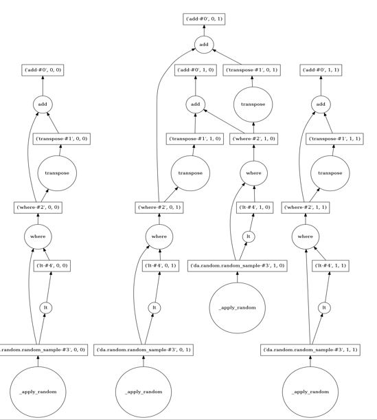
Figure 3.  Task graph for x+x.T with 2×2 chunking of data

The second step for Dask is to send the graph to the scheduler to schedule the subtasks and execute them on the available resources. That step is accomplished with a call to the compute method.

y.compute()

Dask arrays support almost all the standard numpy array operations except those that involve complex communications such as sorting.

In addition to numpy-style arrays, Dask also has a feature called Dask dataframes that are distributed versions of Pandas dataframes.   In this case each Dask dataframe is partitioned by blocks of rows where each block is an actual Pandas dataframe.  In other words, Dask dataframes operators are wrappers around the corresponding Pandas wrappers in the same way that Dask array operators are wrappers around the corresponding numpy array operators.    The parallel work is done primarily by the local Pandas and Numpy operators working simultaneously on the local blocks and this is followed by the necessary data movement and computation required to knit the partial results together.  For example, suppose we have a dataframe, df, where each row is a record consisting of a name and a value and we would like to compute the sum of the values associated with each name.   We assume that names are repeated so we need to group all records with the same name and then apply a sum operator.  We set this up on a system with three workers.  To see this computational graph we write the following.

df.groupby(['names']).sum().visualize()

groupby

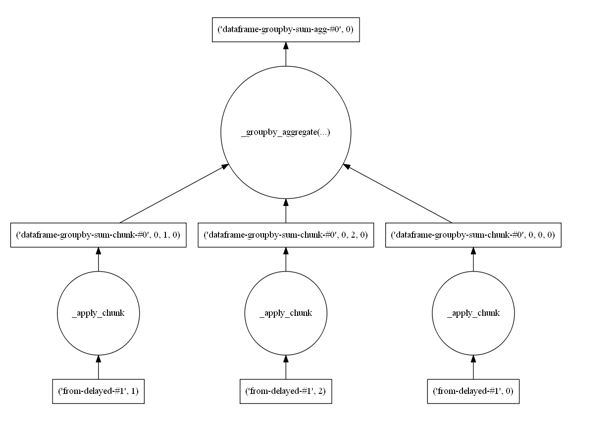
Figure 4.  Dataframe groupby reduction

As stated earlier, one of the motivations of Dask is the ability to work with data collections that are far too large to load on to your local machine.   For example, consider the problem of loading the New York City taxi data for an entire year.    It won’t fit on my laptop.   The data for is for 245 million passenger rides and contains a wealth of information about each ride.  Though we can’t load this into our laptop we can ask dask to load it from a remote repository into our cloud and automatically partition it using the read_csv function on the distrusted dataframe object as shown below.

taxi1

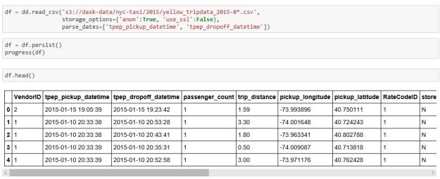
Figure 5.  Processing Yellow Cab data for New York City

The persist method moves the dataframe into memory as a persistent object that can be reused without being recomputed.  (Note:  the read_cvs method did not work on our kubernetes clusters because of a missing module s3fs in the dask container, but it did work on our massive shared memory VM which has 200 GB of memory.)

Having loaded the data we can now follow the dask demo example and compute the best hour to be a taxi driver based on the fraction of tip received for the ride.

taxi3

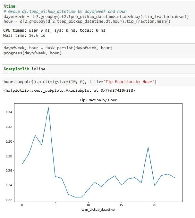
Figure 6.  New York City cab data analysis.
As you can see, it is best to be a taxi driver about 4 in the morning.

A more general distributed data structure is the Dask Bag that can hold items of less structured type than array and dataframes.   A nice example http://dask.pydata.org/en/latest/examples/bag-word-count-hdfs.html illustrates using Dask bags to explore the Enron public email archive.

Dask Futures and Delayed

One of the more interesting Dask operators is one that implements a version of the old programming language concept of a future   A related concept is that of lazy evaluation and this is implemented with the dask.delayed function.   If you invoke a function with the delayed operator it simply builds the graph but does not execute it.  Futures are different.    A future is a promise to deliver the result of a computation later.  The future computation begins executing but the calling thread is handed a future object which can be passed around as a proxy for the result before the computation is finished.

The following example is a slightly modified version of one of the demo programs.   Suppose you have four functions

def foo(x):
   return result
def bar(x):    
   return result
def linear(x, y):
   return result
def three(x, y, z):
   return result

We will use the distributed scheduler to illustrate this example. We first must create a client for the scheduler. Running this on our Azure Kubernetes cluster we get the following.

 
from dask.distributed import Client
c = Client()
c

azure-scheduler

To illustrate the delayed interface, let us build a graph that composes our example functions

from dask import visualize, delayed
i = 3
x = delayed(foo)( I )
y = delayed(bar)( x )
z = delayed(linear)(x, y)
q = delayed(three)( x, y, z)
q.visualize(rankdir='LR')

In this example q is now a placeholder for the graph of a delated computation.   As with the dask array examples, we can visualize the graph (plotting it from Left to Right).

delayed-graph

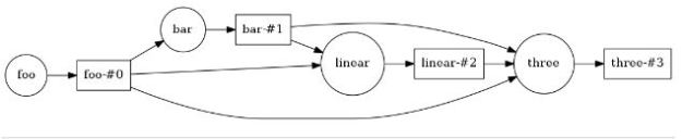
Figure 7.  Graph of a delayed computation.

A call to compute will evaluate our graph.   Note that we have implemented the  four functions each with about 1 second of useless computational math (computing the sum of a geometric series) so that we can measure some execution times.   Invoking compute on our delayed computation gives us

delayed_result

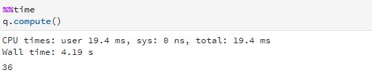
which shows us that there is no parallelism exploited here because the graph has serial dependences.

To create a future, we “submit” the function and its argument to the scheduler client.  This immediately returns a reference to future value and starts the computation.  When you need the result of the computation the future has a method “result()” that can be invoked and cause the calling thread to wait until the computation is done.

Now let us consider the case where the we need to evaluate this graph on 200 different values and then sum the results.   We can use futures to kick off a computation for each instance and wait for them to finish and sum the results.   Again, following the example in the Dask demos, we ran the following on our Azure Kubernetes cluster:

futures-azure-result

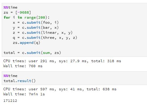
Ignore the result of the computation (it is correct). The important result is the time. Calculating the time to run this sequentially (200*4.19 = 838 seconds) and dividing by the parallel execution time we get a parallel speed-up of about 2, which is not very impressive. Running the same computation on the AWS Kubernetes cluster we get a speed-up of 4. The Azure cluster has 6 cores and the AWS cluster has 12, so it is not surprising that it is twice as fast. The disappointment is that the speed-ups are not closer to 6 and 12 respectively.

aws48-future

Results with AWS Kubernetes Cluster

However, the results are much more impressive on our 48 core AWS virtual machine.

aws48-future2

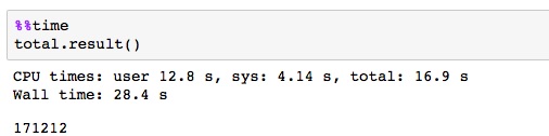
Results with AWS 48-core VM

In this case we see a speed-up of 24.   The difference is the fact that the scheduling is using shared memory and threads.

Dask futures are a very powerful tool when used correctly.   In the example above, we spawned off 200 computations in less than a second.   If the work in the individual tasks is large, that execution time can mask much of the overhead of scheduler communication and the speed-ups can be much greater.

Dask Streams

Dask has a module called streamz that implements a basic streaming interface that allows you to compose graphs for stream processing.   We will just give the basic concepts here.   For a full tour look at https://streamz.readthedocs.io.   Streamz graphs have sources,  operators and sinks.   We can start by defining some simple functions as we did for the futures case:

def inc(x):
    return x+13
def double(x):
    return 2*x
def fxy(x): #expects a tuple
    return x[0]+ x[1]
def add(x,y):
return x+y
from streamz import Stream
source = Stream()

The next step will be to create a stream object and compose our graph.   We will describe the input to the stream later.   We use four special stream operators here.    Map is how we can attach a function to the stream.   We can also merge two streams with a zip operator.   Zip waits until there is an available object on each stream and then creates a tuple that combines both into one object.   Our function fxy(x) above takes a tuple and adds them.   We can direct the output of a stream to a file, database, console output or another stream with the sink operator.  Shown below our graph has two sink operators.

stream1

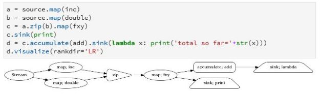
Figure 8.  Streamz stream processing pipeline.

Visualizing the graph makes this clear.   Notice there is also an accumulate operator.   This allows state flowing through the stream to be captured and retained.   In this case we use it to create a running total.  To push  something into the stream we can use the emit() operator as shown below.

stream2

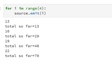
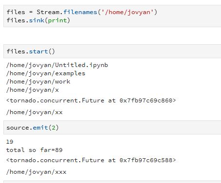
The emit() operator is not the only way to send data into a stream. You can create the stream so that it takes events from kafka, or reads lines from a file or it can monitor a file system directory looking for new items. To illustrate that we created another stream to look at the home director of our kubernetes cluster on Azure. Then we started this file monitor. The names of the that are there are printed. Next, we added another file “xx” and it picked it up. Next, we invoked the stream from above and then added another file “xxx”.

stream3

Handling Streams of Big Tasks

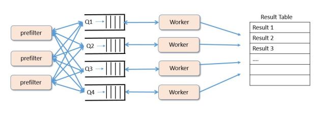
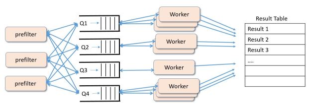
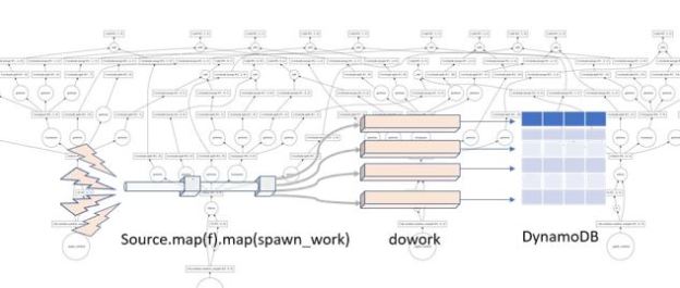
Of the five types of parallel programming Dask covers 2 and a half:  many task parallelism, map-reduce and bulk synchronous parallelism and part of graph dataflow.   Persistent microservices  are not part of the picture.   However, Dask and Streamz can be used together to handle one of the use cases for microservices.  For example, suppose you have a stream of tasks and you need to do some processing on each task but the arrival rate of tasks exceed the rate at which you can process them.   We treated this case with Microservices while processing image recognition with MxNet and the resnet-152 deep learning model (see this article.)  One can  use the Streams sink operation to invoke a future to spawn the task on the Kubernetes  cluster.   As the tasks finish the results can be pushed to other processes for further work or to a table or other storage as illustrated below.

process-events

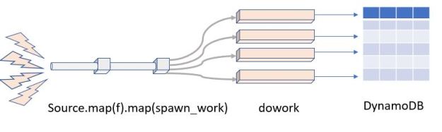
Figure 9 Extracting parallelism from a stream.

In the picture we have a stream called Source which gathers the events from external sources.  We then map it to a function f() for initial processing. The result of that step is sent to a function called spawn_work which creates a future around a function that does some deep processing and sends a final result to an AWS DynamoDB table.   (The function putintable(n) below shows an example.  It works by invoking a slow computation then create the appropriate DynamoDB metadata and put the item in the table “dasktale”.)

def putintable(n): 
    import boto3 
    e = doexp(n*1000000) 
    dyndb = boto3.resource('dynamodb', … , region_name='us-west-2' )
    item ={'daskstream':'str'+str(n),'data': str(n), 'value': str(e)} 
    table = dyndb.Table("dasktale") 
    table.put_item(Item= item ) 
    return e 

def spawn_work(n): 
    x = cl.submit(putintable, n)

This example worked very well. Using futures allowed the input stream to work at full speed by exploiting the parallelism. (The only problem is that boto3 needs to be installed on all the kubernetes cluster processes. Using the 48 core shared memory machine worked perfectly.)
Dask also has a queue mechanism so that results from futures can be pushed to a queue and another thread can pull these results out. We tried as well, but the results were somewhat unreliable.

Conclusion

There are many more stream, futures, dataframe and bag operators that are described in the documents.   While it is not clear if this stream processing tool will be robust enough to replace any of the other systems current available, it is certainly a great, easy-to-use teaching tool.   In fact, this statement can be made about the entire collection of Dask related tools.   I would not hesitate to use it in an undergraduate course on parallel programming.   And I believe that Dask Dataframes technology is very well suited to the challenge of big data analytics as is Spark.

The example above that uses futures to extract parallelism from a stream challenge is interesting because it is completely adaptive. However, it is essential to be able to launch arbitrary application containers from futures to make the system more widely applicable.   Some interesting initial work has been done on this at the San Diego Supercomputer center using singularity to launch jobs on their resources using Dask.   In addition the UK Met Office is doing interesting things with autoscaling dask clusters.   Dask and StreamZ are still young.   I expect them to continue to evolve and mature in the year ahead.

CNTK Revisited. A New Deep Learning Toolkit Release from Microsoft

In a pair of articles from last winter (first article, second article) we looked at Microsoft’s “Computational Network Toolkit” and compared it to Google’s Tensorflow.   Microsoft has now released a major upgrade of the software and rebranded it as part of the Microsoft Cognitive Toolkit.  This release is a major improvement over the initial release.  Because these older articles still get a fair amount of web traffic we wanted to provide a proper update.

There are two major changes from the first release that you will see when you begin to look at the new release.   First is that CNTK now has a very nice Python API and, second, the documentation and examples are excellent.   The core concepts are the same as in the initial release.   The original programming model was based on configuration scripts and that is still there, but it has been improved and renamed as “Brain Script”.  Brain Script is still an excellent way to build custom networks, but we will focus on the Python API which is very well documented.

Installing the software from the binary builds is very easy on both Ubuntu Linux and Windows.   The process is described in the CNTK github site.    On a Linux machine, simply download the gziped tared binary and execute the installer.

$wget https://cntk.ai/'BinaryDrop/CNTK-2-0-beta2-0-Linux-64bit-CPU-Only.tar.gz’
$tar -xf CNTK-2-0-beta2-0-Linux-64bit-CPU-Only.tar.gz
$cd cntk/Scripts/linux
$./install-cntk.sh

This will install everything including a new version of Continuum’s Anaconda Python distribution.  It will also create a directory called “repos’’.   To start Jupyter in the correct conda environment do the following.

$source “your-path-to-cntk/activate-cntk"
$cd ~/repos/cntk/bindings/python/tutorials
$Jupyter notebook 

A very similar set of commands will install CNTK on your Windows 10 box. (If you are running Jupyter on a virtual machine or in the cloud you will need additional arguments to the Jupyter notebook command such as “-ip 0.0.0.0 –no browser” and then then you can navigate you host browser to the VM ip address and port 8888. Of course, if it is a remote VM you should add a password. ) What you will see is an excellent set of tutorials as shown in Figure 1.

jupyter-cntk

Figure 1.   CNTK tutorial Jupyter notebooks.

CNTK Python API

CNTK is a tool for building networks and the Python and Brain Script bindings are very similar in this regard.   You use the Python program to construct a network of tensors and then train and test that network through special operations which take advantage of underlying parallelism in the hardware such as multiple cores or multiple GPUs.   You can load data into the network through Python Numpy arrays or files.

The concept of constructing a computation graph for later execution is not new.   In fact, it is an established programming paradigm used in Spark, Tensorflow, and Python Dask.   To illustrate this in CNTK consider the following code fragment that creates two variables and a constructs a trivial graph that does matrix vector multiplication and vector addition.  We begin by creating three tensors that will hold the input values  to the graph and then tie them to the matrix multiply operator and vector addition.

import numpy as np
import cntk
X = cntk.input_variable((1,2))
M = cntk.input_variable((2,3))
B = cntk.input_variable((1,3))
Y = cntk.times(X,M)+B

In this X is a 1×2 dimensional tensor, i.e. a vector of length 2 and M is a matrix that is 2×3 and B is a vector of length 3. The expression Y=X*M+B yields a vector of length 3. However, no computation has taken place. We have only constructed a graph of the computation. To invoke the graph we input values for X, B and M and then apply the “eval’’ operator on Y. We use Numpy arrays to initialize the tensors and supply a dictionary of bindings to the eval operator as follows

x = [[ np.asarray([[40,50]]) ]]
m = [[ np.asarray([[1, 2, 3], [4, 5, 6]]) ]]
b = [[ np.asarray([1., 1., 1.])]]

print(Y.eval({X:x, M: m, B: b}))
array([[[[ 241.,  331.,  421.]]]], dtype=float32)

CNTK has several other important tensor containers but two important ones are

  • Constant(value=None, shape=None, dtype=None, device=None, name=”): a scalar, vector or other multi-dimensional tensor.
  • Parameter(shape=None, init=None, dtype=None, device=None, name=”): a variable whose value is modified during network training.

There are many more tensor operators and we are not going to go into them here.   However, one very important class is the set of operators that can be used to build multilevel neural networks.   Called the “Layers Library’’ they form a critical part of CNTK.    One of the most basic is the Dense(dim) layer which creates a fully connected layer of output dimension dim. As shown in Figure 2.

cntk-dense

Figure 2.   A fully connected layer created by the Dense operator with an implicit  3×6 matrix and a 1×6 vector of parameters labeled here M and B.   The input dimension is taken from the input vector V.  The activation here is the default (none), but it could be set to ReLu or Sigmod or another function.

There are many standard layer types including Convolutional, MaxPooling, AveragePooling and LSTM. Layers can also be stacked with a very simple operator called “sequential’’. Two examples taken directly from the documentation is a standard 4 level image recognition network based on convolutional layers.

with default_options(activation=relu):
    conv_net = Sequential ([
        # 3 layers of convolution and dimension reduction by pooling
        Convolution((5,5), 32, pad=True), MaxPooling((3,3), strides=(2,2)),
        Convolution((5,5), 32, pad=True), MaxPooling((3,3), strides=(2,2)),
        Convolution((5,5), 64, pad=True), MaxPooling((3,3), strides=(2,2)),
        # 2 dense layers for classification
        Dense(64),
        Dense(10, activation=None)
    ])

The other fun example is a slot tagger based on a recurrent LSTM network.

tagging_model = Sequential ([
    Embedding(150),         # embed into a 150-dimensional vector
    Recurrence(LSTM(300)),  # forward LSTM
    Dense(labelDim)         # word-wise classification
])

The Sequential operator can be thought of as a concatenation of the layers that in the given sequence.   In the case of the slot tagger network, we see two additional important operators: Embedding and Recurrence.

Embedding is used for word embeddings where the inputs are sparse vectors of size equal to the word vocabulary (item i = 1 if the word is the i-th element of the vocabulary and 0 otherwise) and the embedding matrix is of size vocabulary-dimension by, in this case, 150.     The embedding matrix may be passed as a parameter or learned as part of training.

The Recurrence operator is used to wrap the correct LSTM output back to the input for the next input to the network.

A Closer Look at One of Tutorials.

The paragraphs above are intended to give you the basic feel of what CNTK looks like with its new Python interface.  The best way to learn more is to study the excellent example tutorials.

CNTK 203: Reinforcement Learning Basics

CNTK version 1 had several excellent tutorials, but version 2 has the Python notebook versions of these plus a few new ones.  One of the newest demos is an example of reinforcement learning.   This application of Neural Nets was first described in the paper Human-level control through deep reinforcement learning, by the Google DeepMind group.  This idea has proven to be very successful in systems that learn to play games.  This topic has received a lot of attention, so we were happy to see this tutorial included in CNTK. The example is a very simple game that involves balancing a stick.   More specifically they use the cart-pole configuration from OpenAI.   As shown in figure 3, the system state can be described by a 4-tuple: position of the cart, its velocity, the angle of the pole and the angular velocity.   The idea of the game is simple.  You either push the cart to the left or the right and see if you can keep the stick vertical.   If you drift too far off course or the pole angle goes beyond an angle of 15 degrees, the game is over.   Your score is the total number of steps you take before failure. The full example is in the github repository and we are not going to go through all the code here.  The Jupyter notebook for this example is excellent, but if you are new to this topic you may find some additional explanation of value in case you decide to dig into it.cntk-cart-pole

Figure 3. Cart-Pole game configuration.

The part of reinforcement learning used here is called a Deep Q-Network. It uses a neural network to predict the best move when the cart is in a given state. This is done by implicitly modeling a function Q(s,a) which is the optimal future reward given state s and the action is a and where the initial reward is r. They approximate Q(s,a) using the “Bellmann equation” which describes how to choose action a in a given state s to maximize the accumulated reward over time based inductively on the same function applied to the following states s’.

cntk-bellmann

The parameter gamma is a damping factor that guarantees the recurrence converges. (Another excellent reference for this topic is the blog by Jaromír Janisch.) The CNTQ team approached this problem as follows. There are three classes.

  • Class Brain.    This hold our neural net and trainer.  There are three methods
    • Create() which is called at initialization.   It creates the network.   There are two tensor parameters: observation, which is used to hold the input state and q_target which is a tensor used for training.   The network is nice and simple:
      l1 = Dense(64, activation=relu)
      l2 = Dense(2)
      unbound_model = Sequential([l1, l2])
      model = unbound_model(observation)
      

      The training is by the usual stochastic gradient descent based on a loss measure.

      loss = reduce_mean(square(model - q_target), axis=0)
      meas = reduce_mean(square(model - q_target), axis=0)
      learner = sgd(model.parameters, lr,    
             gradient_clipping_threshold_per_sample=10)
      trainer = Trainer(model, loss, meas, learner)
      
    • Train(x, y)  which calls the trainer for batches of states x and predicted outcomes y which we will describe below
    • Predict(s) which invokes the model for state ‘s’ and returns a pair of optimal rewards given a left or right move.
  • Class Memory. This hold a record of recent moves.   This is used by the system to create training batches.  There are two methods
    • Add(sample configuration)  – adds a four tuple consisting of a starting state, an action and a result and a resulting  state tuple to a memory.
    • Sample(n) returns a random sample of n configurations samples from the memory.
  • Class Agent which is the actor that picks the moves and uses the memory to train the network.  There are three methods here.
    • Act(state) returns a 0 or 1 (left move or right move) that will give the best reward for the given state.     At first it just makes random guesses, but as time passes it uses the Predict method of the Brain class to select the best move for the given state.
    • Observe(sample configuration) records a configuration in the memory and keeps track of the time step and another parameter used by act.
    • Replay() is the main function for doing the learning.    This is the hardest part to understand in this tutorial. It works by grabbing a random batch of memorized configurations from memory.   What we will do is use the current model to predict an optimal outcome and use that as the next step in training the model.  More specifically for each tuple in the batch we want to turn it into a training sample so that the network behaves like the Bellmann equation.  A tuple consists of the start state, the action, the reward and the following state.   We can apply our current model to predict the award for the start state and also for the result state.  We can use this information to create a new reward tuple for the given action and start state that models the Bellmann recurrence.   Our training example is the pair consisting of the start state and this newly predicted reward.  At first this is a pretty poor approximation, but amazingly over time it begins to converge. The pseudo code is shown below.
      x = numpy.zeros((batchLen, 4)).astype(np.float32)
      y = numpy.zeros((batchLen, 2)).astype(np.float32)
      
      for i in range(batchLen):
          s, a, r, s_ = batch[i]
          # s = the original state (4 tuple)
          # a is the action that was taken
          # r is the reward that was given
          # s_ is the resulting state.
          # let t = the reward computed from current network for s 
          # and let r_ be the reward computed for state s_.
          # now modify t[a] = r + gamma* numpy.amax(r_) 
          # this last step emulated the bellmann equation
          x[i] = s
          y[i] = t
      self.brain.train(x,y)		
      

The final part of the program is now very simple. We have an environment object that returns a new state and a done flag for each action the agent takes. We simply run our agent until it falls out of bounds (the environment object returns done=True). If the step succeeded, we increment our score. The function to run the agent and to keep score is shown below.

def run(agent):
    s = env.reset()
    R = 0 
    while True:            
        a = agent.act(s)
	  s_, r, done, info = env.step(a)
        if done: # terminal state
            s_ = None
        agent.observe((s, a, r, s_))
        agent.replay() #learn from the past           
        s = s_
        R += r
        if done:
            return R

Each time we run “run” it learns a bit more.   After about 7000 runs it will take over 600 steps without failure.

The text above is no substitute for a careful study of the actual code in the notebook.  Also, as it is a notebook, you can have some fun experimenting with it.  We did.

Final Thoughts

CNTK is now as easy to use as any of the other deep learning toolkits.   While we  have not benchmarked its performance they claim it is extremely fast and it make good use of multiple GPUs and even a cluster of servers.    We are certain that the user community will enjoy using and contributing to its success.

Citation.

The team that first created CNTK should be cited.   I know there are likely many others that have contributed to the open source release in one way or another, but the following is the master citation.

Amit Agarwal, Eldar Akchurin, Chris Basoglu, Guoguo Chen, Scott Cyphers, Jasha Droppo, Adam Eversole, Brian Guenter, Mark Hillebrand, T. Ryan Hoens, Xuedong Huang, Zhiheng Huang, Vladimir Ivanov, Alexey Kamenev, Philipp Kranen, Oleksii Kuchaiev, Wolfgang Manousek, Avner May, Bhaskar Mitra, Olivier Nano, Gaizka Navarro, Alexey Orlov, Hari Parthasarathi, Baolin Peng, Marko Radmilac, Alexey Reznichenko, Frank Seide, Michael L. Seltzer, Malcolm Slaney, Andreas Stolcke, Huaming Wang, Yongqiang Wang, Kaisheng Yao, Dong Yu, Yu Zhang, Geoffrey Zweig (in alphabetical order), “An Introduction to Computational Networks and the Computational Network Toolkit“, Microsoft Technical Report MSR-TR-2014-112, 2014.

A Brief Look at Google’s Cloud Datalab

Google recently released a beta version of a new tool for data analysis using the cloud called Datalab.  In the following paragraphs we take a brief look at it through some very simple examples.  While there are many nice features of Datalab, the easiest way to describe it would be to say that it is a nice integration of the IPython Jupyter notebook system with Google’s BigQuery data warehouse.  It also integrates standard IPython libraries such as graphics and scikit-learn and Google’s own machine learning toolkit TensorFlow.

To use it you will need a Google cloud account.   The free account is sufficient if you are interested in just trying it out.   You may ask, why do I need a Google account when I can use Jupyter, IPython and TensorFlow on my own resources?    The answer is you can easily access BigQuery on non-trivial sized data collections directly from the notebook running on your laptop.  To get started go to the Datalab home page.   It will tell you that this is a beta version and give you two choices: you may either install the Datalab package locally on your machine or you may install it on a VM in the Google cloud.   We prefer the local version because it saves your notebooks locally.

 The Google public data sets that are hosted in the BigQuery warehouse are fun to explore.  They include

  • The names on all US social security cards for births after 1879.  (The table rows contain only the year of birth, state, first name, gender and number as long as it is greater than 5.  No social security numbers.),
  • The New York City Taxi trips from 2009 to 2015,
  • All stories and comments from “Hacker News”,
  • The US Dept of Health weekly records of diseases reported from each city and state from 1888 to 2013,
  • The public data from the HathiTrust and the Internet Book Archive,
  • The global summary of the day’s (GSOD) weather from the national oceanographic and atmospheric administration from 9000 weather stations between 1929 and 2016.

And more, including the 1000 genome database.

To run Datalab on your laptop you need to have Docker installed.   Once Docker is running then and you have created a Google cloud account and created a project, you can launch Datalab with simple docker command as illustrated in their quick-start guide.  When the container is up and running you can view it at http://localhost:8081.  What you see at first is shown in Figure 1.  Keep in mind that this is beta release software so you can expect it will change or go away completely. 

 datalab-first-view

Figure 1.  Datalab Top level view.

Notice the icon in the upper right corner consisting of a box with an arrow.   Clicking this allows you to login to the Google cloud and effectively giving your authorization to allow you container to run on your gcloud account.

The view you see is the initial notebook hierarchy.   Inside docs is a directory called notebooks that contain many great tutorials and samples.

A Few Simple Examples of Using Datalab

As mentioned above, one of the public data collections is the list of first names from social security registrations.   Using Datalab we can look at a sample of this data by using one of the built-in Bigquery functions as shown in Figure 2.

datalab-names

Figure 2.   Sampling the names data.


This page gives us enough information about the schema that we can now formulate a query.

In modern America there is a movement to “post-gender” names.   Typical examples cited on the web are “Dakota”, “Skyler” and  “Tatum”.   A very simple SQL query can be formulated to see how the gender breakdown for these names show up in the data.  In Datalab, we can formulate the query as shown in Figure 3.

datalab-dakotaplus2

Figure 3.   Breakdown by gender of three “post-gender” names.

As we can see, this is very nearly gender balanced.  A closer inspection using each of the three names separately show that “Skyler” tends to be ‘F’ and “Tatum” tends to ‘M’. On the other hand, “Dakota” does seem to be truly post-gender with 1052 ‘F’ and 1200 ‘M’ occurrences.

We can also consider the name “Billy” which, in the US, is almost gender neutral.   (Billy Mitchel was a famous World Work I general and also a contemporary Jazz musician.  Both male. And Billy Tipton and Billy Halliday were female musicians though Billy Halliday was actually named Billie and Billy Tipton lived her life as a man, so perhaps they don’t count.   We can ask how often Billy was used as a name associated with gender ‘F’ in the database?  It turns out it is most common in the southern US. We can then group these by state and create a count and show the top five.   The SQL command is easily inserted into the Datalab note book as shown in Figure 4.

datalab-billy

Figure 4.   Search for Billy with gender ‘F’ and count and rank by state of birth.

Rubella in Washington and Indiana

 A more interesting data collection is Center for Disease Control and Prevention dataset concerning diseases reported by state and city over a long period.   An interesting case is Rubella, which is virus also known as the “German measles”.   Through our vaccination programs it has been eliminated in the U.S. except for those people who catch it in other countries where it still exists.  But in the 1960s it was a major problem with an estimated 12 million cases in the US and a significant number of newborn deaths and birth defects.   The vaccine was introduced in 1969 and by 1975 the disease was almost gone.   The SQL script shown below is a slight modified version of one from the Google Bigquery example.   It has been modified to look for occurrences of Rubella in two states, Washington and Indiana, over the years 1970 and 1971.

%%sql --module rubella
SELECT
  *
FROM (
  SELECT
    *, MIN(z___rank) OVER (PARTITION BY cdc_reports_epi_week) AS z___min_rank
  FROM (
    SELECT
      *, RANK() OVER (PARTITION BY cdc_reports_state ORDER BY cdc_reports_epi_week ) AS z___rank
    FROM (
      SELECT
        cdc_reports.epi_week AS cdc_reports_epi_week,
        cdc_reports.state AS cdc_reports_state,
        COALESCE(CAST(SUM((FLOAT(cdc_reports.cases))) AS FLOAT),0) 
         AS cdc_reports_total_cases
      FROM
        [lookerdata:cdc.project_tycho_reports] AS cdc_reports
      WHERE
        (cdc_reports.disease = 'RUBELLA')
        AND (FLOOR(cdc_reports.epi_week/100) = 1970 
          OR FLOOR(cdc_reports.epi_week/100) = 1971)
        AND (cdc_reports.state = 'IN'
          OR cdc_reports.state = 'WA')
      GROUP EACH BY
        1, 2) ww ) aa ) xx
WHERE
  z___min_rank <= 500
LIMIT
  30000

We can now invoke this query as part of a python statement so we can capture its result as a pandas data frame and pull apart the time stamp fields and data values.

rubel = bq.Query(rubella).to_dataframe()
rubelIN = rubel[rubel['cdc_reports_state']=='IN']
                 .sort_values(by=['cdc_reports_epi_week'])
rubelWA = rubel[rubel['cdc_reports_state']=='WA']
                 .sort_values(by=['cdc_reports_epi_week'])
epiweekIN = rubelIN['cdc_reports_epi_week']
epiweekWA = rubelWA['cdc_reports_epi_week']
rubelINval = rubelIN['cdc_reports_total_cases']
rubelWAval = rubelWA['cdc_reports_total_cases']

At this point a small adjustment must be made to the time stamps.  The CDC reports times in epidemic weeks and there are 52 weeks in a year.    So the time stamps for the first week of 1970 is 197000 and the time stamp for the last week is 197051.  The next week is 197100.  To make these into timestamps that appear contiguous we need to make a small “time compression” as follows.

realweekI = np.empty([len(epiweekIN)])
realweekI[:] = epiweekIN[:]-197000
realweekI[51:] = realweekI[51:]-48

Doing the same thing with epiweekWA we now have the basis of something we can graph.  Figure 5 shows the progress of rubella in Washington and Indiana over two years.  Washington is the red line and Indiana is blue.   Note that the outbreaks occur about the same time in both states and that by late 1971 the disease is nearly gone.

datalab-rubella.png

Figure 5.   Progress of Rubella in Washington (red) and Indiana (blue) from 1970 through 1971.

Continuing the plot over 1972 and 1973 show there are flare-ups of the disease each year but their maximum size is diminishes rapidly.

(Datalab has some very nice plotting functions, but we could not figure out how to do a double plot, so we used the mathplot library with the “fivethirtheight” format.)


A Look at the Weather


From the national oceanographic and atmospheric administration we have the global summary of the day’s (GSOD) weather from the from 9000 weather stations between 1929 and 2016.   While not all of these stations were operating during that entire period, there is still a wealth of weather data here.   To illustrate it, we can use another variation on one of Google’s examples.  Let’s find the hottest spots in the state of Washington for 2015.   This was a particularly warm year that brought unusual droughts and fires to the state. The following query will list the hottest spots in the state for the year.

%%sql
SELECT
  max, (max-32)*5/9 celsius, mo, da, state, stn, name
FROM (
  SELECT
    max, mo, da, state, stn, name
  FROM
    [bigquery-public-data:noaa_gsod.gsod2015] a
  JOIN
    [bigquery-public-data:noaa_gsod.stations] b
  ON
    a.stn=b.usaf
    AND a.wban=b.wban
  WHERE
    state="WA"
    AND max

 The data set ‘gsod2015’ is the table of data for the year 2015.  To get a list that also shows the name of the station we need to do a join with the ‘station’ table over the corresponding station identifiers.  We order the results descending from the warmest recordings.    The resulting table is shown in Figure 6 for the top 10.

datalab-hotstations

Figure 6.   The top 10 hottest spots in Washington State for 2015

The results are what we would expect.   Walla Walla, Moses Lake and Tri Cities are in the eastern part of the state and summer was very hot there in 2015.   But  Skagit RGNL is in the Skagit Valley near Puget Sound.   Why is it 111 degrees F there in September?   If it is hot there what was the weather like in the nearby locations?   To find out which stations were nearby we can look at the stations on a map.   The query is simple but it took some trial and error.

%%sql --module stationsx
DEFINE QUERY locations
  SELECT FLOAT(lat/1000.0) AS lat, FLOAT(lon/1000.0) as lon, name
  FROM [bigquery-public-data:noaa_gsod.stations]
  WHERE state="WA" AND name != "SPOKANE NEXRAD"

It seems that the latitude and longitude for the Spokane NEXRAD station are incorrect and resolve to some point in Mongolia.  By removing it we get a good picture of the nearby stations as shown in Figure 7.

datalab-hotstations.png

Figure 7.   Location of weather stations in western Washington using the Bigquery chart map function.

 This is an interactive map, so we can get the names of the nearby stations.   There is one only a few miles away  called PADILLA BAY RESERVE and the next closest is BELLINGHAM INTL.   We can now compare the weather for 2015 at these three locations.

 To get the weather for each of these we need the station ID.   We can do that with a simple query.

%%sql
SELECT
  usaf, name
FROM [bigquery-public-data:noaa_gsod.stations] 
WHERE
    name="BELLINGHAM INTL" OR name="PADILLA BAY RESERVE" OR name = "SKAGIT RGNL"

Once we have our three station IDs we can use the follow to build a parameterized Bigquery expression.

qry = "SELECT max AS temperature, \
       TIMESTAMP(STRING(year) + '-' + STRING(mo) + \
       '-' + STRING(da)) AS timestamp \
FROM [bigquery-public-data:noaa_gsod.gsod2015] \
WHERE stn = '%s' and max /< 500 \
ORDER BY year DESC, mo DESC, da DESC"

stationlist = ['720272','727930', '727976']

dflist = [bq.Query(qry % station).to_dataframe() for station in stationlist]

 We can now render an image of the weather for our three stations as shown in Figure 8.

datalab-3stations-final.png

Figure  8.  Max daily temperatures for Skagit (blue), Padilla Bay (red) and Bellingham (yellow)

 We can clearly see the anomaly for Skagit in September and it is also easy to spot another problem in March where the instruments seemed to be not recording.   Other than that there is close alignment of the readings.

Conclusions

There are many features of Datalab that we have not demonstrated here.   The documentation gives an example of using Datalab with Tensorflow and the charting capabilities are more extensive than demonstrated here.  (The Google maps example here was not reproducible in any other notebook beyond the demo in the samples which we modified to run the code here.)  It is also easy to upload your own data to the warehouse and analyze it with Datalab.

 Using Datalab is almost addictive.  For every one of the data collections we demonstrated here there were many more questions we wanted to explore.  For example, where and when did the name “Dakota” start being used and how did its use spread?   Did the occurrence of Rubella outbreaks correspond to specific weather events?  Can we automate the process of detecting non-functioning weather instruments over the years where records exist?  These are all relatively standard data mining tasks, but the combination of Bigquery and IPython in the notebook format makes it fun.

 It should be noted that Datalab is certainly not the first use of the IPython notebook as a front-end to cloud hosted analysis tools.  The IPython notebook has been used frequently with Spark as we have previously described.  Those interested in an excellent overview of data science using Python should look at “Python Data Science Handbook”  by Jake VanderPlas which makes extensive use of IPython notebooks.     There are a variety of articles about using Jupyter on AWS  and Azure for data analytics.  A good one is by Cathy Ye about deep learning using Jupyter in the cloud where she gives detailed instruction for how to install Jupyter on AWS and deploy Caffe there.

.

Kubernetes and the Google Cloud Container Service: Fun with Pods of Celery.

In a previous post I talked about using Mesosphere on Azure for scaling up many-tasks parallel jobs and I promised to return to Kubernetes when I figured out how to bring it up.   Google just made it all very simple with their new Google Cloud container services.   And, thanks to their good tutorials, I learned about a very elegant way to do remote procedure calls using another open source tool called Celery.

So let me set the stage with a variation on an example I have used in the past.   Suppose we have 10000 scientific documents that are stored in the cloud.   I would like to use a simple machine learning method to classify each of these by topic.    I would like to do this quickly as possible and, because the analysis of each document is independent of the others, I can try to process as many as possible in parallel.  This is the basic “many task” parallel model and one of the most common uses of the cloud for scientific computing purposes.      To do this we will use the Celery distributed task queue mechanism to take a list of our documents and send each one to a work queue where the tasks will be parceled out to workers who will do the analysis and respond.

The Google Cloud Container Service and a few words about Kubernetes.

Before getting into the use of Celery and the analysis program, let’s describe the Google Cloud Container Service and a bit about Kubernetes.   Getting started is incredibly easy.   Google has a small free trial account which is sufficient to do the experiments described.  Go to http://cloud.google.com and sign in or create an account.  This will take you to the “console” portal. The first thing you need to do is to create a project. In doing so it will be assigned an id which is a string of the form “silicon-works-136723”.    There is a drop down menu on the left end of the blue banner at the top of the page.  (Look for three horizontal bars.) This allows you to select the type of service you want to work on.     Select the “Container Engine”.  On the “container clusters” page there is a link that will allow you to create a cluster.   With the free account you cannot make a very big cluster.   You are limited to about 4 dual core servers.   If you fill in the form and submit it, you will soon have a new cluster.  There is a special icon of the form “>_” in the blue banner.  Clicking on that icon will create an instance of a “Cloud Shell” that will be automatically authenticated to your account.   The page you will see should resemble Figure 1 below.   The next thing you need to do is to authenticate your cloud shell with your new cluster.   By selecting your container and clicking on the “connect” button to the right you will get the code to paste into the cloud shell.  The result should now look exactly like Figure 1.

google-container-engine

Figure 1.   Creating a Google cloud cluster and connecting the cloud shell to it.

Interacting with Kubernetes, which is now running on our small cluster, is through command lines which can be entered into the cloud shell.   Kubernetes has a different, and somewhat more interesting architectures than other container management tools.   The basic unit of scheduling in Kubernetes is  launching pods. A pod consists of a set of one or more Docker-style containers together with a set of resources that are shared by the containers in that pod.  When launched a pod resides on a single server or VM.   This has several advantages for the containers in that pod.   For example, because the containers in a pod are all running  on the same VM, the all share the same IP and port space so the containers can find each other through conventional means like “localhost”.   They can also share storage volumes that are local to the pod.

To start let’s consider a simple single container pod to run the Jupiter notebook.  There is a standard Docker container that contains Jupyter and the scipy software stack.  Using the Kubernetes control command kubectl we can launch Jupyter and expose its port 8888 with the following statement.

$ kubectl run jupyter --image=jupyter/scipy-notebook --port=8888

To see that it is up and running we can issue the command “kubectl get pods” which will return the status of all of our running pods.   Though we have launched jupyter it is still not truly visible.   To do that we will associate a load balancer with the pod.   This will expose the port 888 to the open Internet.

$ kubectl expose deployment jupyter --type=LoadBalancer

Once that has been run you can get the IP address for jupyter from the “LoadBalancer Ingress:” field of the service description when you run the following.   If it doesn’t appear, try again.

$ kubectl describe services jupyter

One you have verified that it is working at that address on port 8888, you should shut it down immediately because, as you can see, there is no security with this deployment.  Deleting a deployment is easy.

$ kubectl delete deployment jupyter

 There is another point that one must be aware of when building containers that need to directly interact with the google cloud APIs.  To make this work you will need to get application default credentials to run in your container.   For example if you container is going to interact with the storage services you will need this.   To get the default application credentials follow the instructions here.  We will say a few more words about this below.

The Analysis Example in detail.

Now to describe  Celery and how to use Celery and Kubernetes in the many-task scenario described above.

To use Celery we start with our analysis program.   We have previously described the analysis algorithms in detail in another post, so we won’t duplicate that here.  Let’s start by assuming we have a function predict(doc) that takes a document as a string as an argument and returns a string containing the result from our trained machine learnging classifiers.  Our categories are “Physics”, “Math”, “Bio”, “Computer Science” and “Finance” and the result from each classifier is simply the category that that classifier determines to be the most likely correct answer.

Celery is a distributed remote procedure call system for Python programs.   The Celery view of the world is you have a set of worker processes running on remote machines and a client process that is invoking functions that are executed on the remote machines.   The workers and the clients all coordinate through a message broker running somewhere else on the network.

Here we use a RabbitMQ service that is running on a Linux VM on the NSF JetStream cloud as illustrated in Figure 2.

kubernetes-jetstream-setup

Figure 2.  Experimental Configuration with Celery workers running on Kubernetes in the Google Cloud Container Service,  the RabbitMQ broker running in a VM on the NSF Jetstream Cloud and a client program running as a notebook on a laptop.

The code block below illustrates the basic Celery worker template.    Celery is initialized with a constructor that takes the name of the project and a link to the broker service which can be something like a Redis cache or MongoDB.   The main Celery magic is invoked with a special Python “decorator” associated with the Celery object as shown in the predictor.py file below.

from celery import Celery
app = Celery('predictor', backend='amqp')

#Now initialize and load all the data structure that will be constant 
#and recused for each analysis.  In our case this will include
#all the machine learning models that were trained on the data 
#previously. And create a main worker function to invoke the models.  
def invokeMLModels(statement):
    ....
	return analysis
	
#define the functions we will call remotely here
@app.task
def predict(statement):
	prediction = invokeMLModels(statement)
	return [prediction]

What this decorator accomplishes is to wrap the function in a manner that it can be invoked by a remote client.   To make this work we need create a Celery worker from our predictor.py file with the command below which registers a worker instance as a listener on the RabbitMQ queue.

>celery worker -A predictor -b 'amqp://guest@brokerIPaddr'

Creating a client program for our worker is very simple.   It is similar to the worker template except that our version of the predict( ) function does nothing because we are going to invoke it with the special Celery apply_async( ) method that will push the argument to the broker queue and return control immediately to the client.   The object that is returned from this call is similar to what is sometimes called a “future” or a “promise” in the programming language literature.  What it is a placeholder for the returned value.   Once we attempt to evaluate the get() method on this object our client will wait until a reply is returned from the remote worker that picked up the task.

from celery import Celery
app = Celery('predictor', broker='amqp://guest@brokerIPaddr', backend='amqp')

@app.task
def predict(statement):
	return ["stub call"]
	
res = predict.apply_async(["this is a science document ..."])

print res.get()

Now if we have 10000 documents to analyze we can send them in sequence to the queue as follows.

#load all the science abstracts into a list
documents = load_all_science_abstracts()

res = []
for doc in documents:
   res.append(predict.apply_async([doc])

#now wait for them all to be done
predictions = [result.get() for result in res]
#now do an analysis of the predictions

Here we push each analysis task into the queue and save the async returned objects in a list.  Then we create a new list by waiting for each prediction value to be returned.   Our client can run anywhere there is Internet access.  For example this one was debugged on a Jupyter instances running on a laptop.  All you need to do is “pip install celery” and run Juypter.

There is much more to say about Celery and the interested reader should look at the Celery Project site for the definitive guide. Let us now turn to using this with Kubernetes.  We must first create a container to hold the analysis code and all the model data.   For that we will need a Docker file and a shell script to correctly launch celery one the container is deployed.   For those actually interested in trying this, all the files and data are in OneDrive here.   The Docker file shown below has more than we need for this experiment.

# Version 0.1.0
FROM ipython/scipystack
MAINTAINER yourdockername "youremail"
RUN easy_install celery
RUN pip install -U Sphinx
RUN pip install Gcloud
RUN easy_install pattern
RUN easy_install nltk
RUN easy_install gensim
COPY bookproject-key.json /
COPY models /
COPY config /
COPY sciml_data_arxiv.p /
COPY predictor.py /
COPY script.sh /
ENTRYPOINT ["bash", "/script.sh"]

To build the image we first put all the machine learning configuration files in a directory called config and all the learned model files in a directory called models.  At same level we have the predictor.py source.   For reasons we will explain later we will also include the full test data set: sciml_data_arxiv.p. The Docker build starts with the ipython/scipystack container.   We then use easy_install to install Celery as well as four packages used by the ML analyzers: pattern, nltk and gensim.   Though we are not going to use the Gcloud APIs here, we include them with a pip install.   But to make that work we need an updated copy of Sphinx.  To make the APIs work we would need our default client authentication keys.   They are stored in a json file called bookproject-key.json that was obtained from the Gcloud portal as described previously.   Finally we copy all of the files and directory to the root path ‘/’.  Note that the copy from a directory is a copy of the all contained files to the path ‘/’ and not to a new directory.   The ENTRYPOINT runs our script which is shown below.

cp /predictor.py .
export C_FORCE_ROOT='true'
export GOOGLE_APPLICATION_CREDENTIALS='/bookproject-key.json'
echo $C_FORCE_ROOT
celery worker -A predictor -b $1

Bash will run our script in a temp directory, so we need to copy our predictor.py file to that directory.  Because our bash is running as root, we need to convince Celery that it is o.k. to do that.  Hence we export C_FORCE_ROOT as true.  Next, if we were using the Gcloud APIs we need to export the application credentials.   Finally we invoke celery but this time we use the -b flag to indicate that we are going to provide the IP address of the RabbitMQ amqp broker as a parameter and we remove it from the explicit reference in the predictor.py file.  When run the predictor file will look for all the model and configuration data in ‘/’.   We can now build the docker image with the command

>docker build -t “yourdockername/predictor” .

And we can test the container on our laptop with

>docker run -i -t “yourdockername/predictor ‘amqp://guest@rabbitserverIP’

Using “-i -t” allows you to see any error output from the container.   Once it seems to be working we can now push the image to the docker hub.   (to use our version directly, just pull dbgannon/predictor)

We can now return to our Google cloud shell and pull a version of the container there.   If we want to launch the predictor container on the cluster, we can do it one at a time with the “kubectl run” command.  However Kubernetes has a better way to do this using a pod configuration file where we can specify the number of pod instances we want to create.  In the file below, which we will call predict-job.json we specify a job name, the container image in the docker hub,   and the  parameter to pass to the container to pass to the shell script.   We also specify the number of pods to create.   In this case that is 6 as identified in the “parallelism” parameter.

apiVersion: batch/v1
kind: Job
metadata:
   name:predict-job
spec:
   parallelism: 6
   template:
        metadata:
            name: job-wq
       spec:
            containers:
                  - name: c
                  image: dbgannon/predictor
                  args: ["amqp://guest@ipaddress_of_rabbitmq_server"]
          restartPolicy: OnFailure

One command in the cloud shell will now launch six pods each running our predictor container.

$kubectl create -f predict-job.json 

Some Basic Performance Observations.

When using many tasks system based on a distributed worker model there are always three primary questions about the performance of the system.

  1. What is the impact of wide-area distribution on the performance?
  2. How does performance scale with the number of worker containers that are deployed? More specifically, if we N workers, how does the system speed up as N increases?    Is there a point of diminishing return?
  3. Is there a significant per/task overhead that the system imposes?  In other words, If the total workload is T and if it is possible to divide that workload into k tasks each  of size T/k , then what is the best value of k that will maximize performance?

Measuring the behavior of a Celery application as a function of the number workers is complicated by a number of factors.   The first concern we had was the impact of widely distributing the computing resources on the overall performance.   Our message broker (RabbitMQ) was running in a virtual machine in Indiana on the JetStream cloud.   Our client was running a Jupyter notebook on a laptop and the workers were primarily on the Midwest Google datacenter and on a few on other machines in the lab.   We compared this to a deployment where all the workers, the message broker and the client notebook were all running together on the Google datacenter.   Much to our surprise there was little difference in performance between the two deployments.   There are two ways to view this result.   One way is to say that the overhead of wide area distribution was not significant.   The other way to say this is that the overhead of wide area distribution was negligible compared to other performance problems.

A second factor that has an impact on performance as a function of the number of workers is the fact that a single Celery worker may have multiple threads that are responding to asynchronous function calls.   While we monitored the execution we noticed that the number of active threads in one worker could change over time. This made performance somewhat erratic.  Celery’s policy is that it will never have more threads than the number of available cores, so to limit the thread variability we ran workers in container pods on VMs with only one core.

Concerning the question of the granularity of the work partitioning we configured the program so that a number of documents could be processed in one invocation and this number could be set remotely.    By taking a set of 1000 documents and a fixed set of workers, we divided the document set into blocks of size K where K ranged from 1 to 100.   In general, larger blocks were better because the number of Celery invocations was smaller, but the difference was not great.   Another factor involved Celery’s scheduling for deciding which worker get the next invocation.   For large blocks this was not the most efficient because this left holes in the execution schedule when workers were occasionally idle while another was over scheduled.   For very small blocks these holes tended to be small.   We found that a value of K=2 gave reasonably consistent performance.

Finally to test scalability we used three different programs.

  1. The document topic predictor described above where each invocation classified two documents.
  2. A simple worker program that does no computation but just sleeps for 10 seconds before returning a “hello world” string.
  3. A worker that computes part of the Euler sequence sum(1/i**2, i=1..n) where n = 109 .   Each worker computes a block of 107 terms of the sequence and the 100 partial results are added together to get the final result  (which approximates pi2/6  to about 7 decimal places).

The document predictor is very computational intensive and uses some rather large data matrices for the trained machine learning models.   The size of these arrays are about 150 megabytes total.  While this does fit in memory, the computation is going to involve a great deal of processor cache flushing and there may be memory paging effects.   The example that computes the Euler sum requires no data other than the starting point index and the size of the block to sum.   It is pure computation and it will have no cache flushing or memory paging effects, but it will keep the CPU very busy.   The “sleep” example leaves the memory and the CPU completely idle.

We ran all three with one to seven workers.   (6 workers using 6 cores from the small Google demo account and one on another other remote machine).    To compare the results, we computed the time for each program on one worker and plotted the speed-up ratio for 2, 3, 4, 5, 6 and 7 workers.   The results are shown in the graphs below.

predictor-euler-sleep

Figure 3.  Performance as speed-up for each of the three applications with up to 7 workers.

As can be seen, the sleeper scales linearly in the number of workers.   In fact, when executed on multi-core machines it is almost super-linear because of the extra threads that can be used.  (It is very easy for a large number of threads to sleep in parallel.)   On the other hand, the predictor and the Euler examples reached a maximum speed up with around five workers.  Adding more worker pods to the servers did not show improvement because these applications are already very compute intensive.    This was a surprise as we expect all three experiments to scale well beyond seven workers.  Adding more worker pods to the servers did not show improvement because these applications are already very compute intensive.   When looking for the cause of this limited performance, we considered the possibility that the RabbitMQ broker was a bottleneck, but our previous experience with it has allowed us to scale applications to dozens of concurrent reader and writers.   We are also convinced that the Google Container Engine performed extremely well and it was not the source of any of these performance limitations. We suspect (but could not prove) that the Celery work distribution and result gathering mechanisms have overheads that limit scalability as the number of available workers grows.

Conclusion

Google has made it very easy to deploy containerized applications using Kubernetes on their cloud container service.  Kubernetes has some excellent architectural features that allow multiple containers to be co-located on a single server within a pod.   We did not have time here to demonstrate this, but their documentation gives some excellent examples.

Celery is an extremely elegant way to do remote procedure calls in Python.  One only needs to define the function and annotate it with a Celery object.   It can then be remotely invoked with an asynchronous call that returns control to the caller.  A future like object is returned.  By calling a special method on the returned object the caller will pause until the remote call completes and the value is provided to the caller.

Our experiments demonstrated that Celery has limited scalability if it is used without modification and with the RabbitMQ message broker.   However, celery has many parameters and it may be possible that the right combinations will improve our results.  We will report any improved results we discover in a later version of this document.

A Quick Dive into Cloud Data Streaming Technology

This is the second part of a two part series about data streaming technology.  The first part is about streaming data in science and this part describes the programming models for several open source cloud based data streaming tools including Spark Streaming, Storm and Heron, Googles Dataflow and Apache Flink.

Introduction

Cloud computing evolved from the massive data centers that were built to handle the “big data” challenges that confronted the designers of on-line services like search and e-mail.    For the most part, data from these services accrued into large collections in the cloud where they could be analyzed by massively parallel, batch computing jobs.   The types of knowledge derived from this analysis is used to improve the services that generated the data in the first place.   For example, data analysis of cloud system log files can yield valuable information about how to improve performance of the cloud system.   Analysis of user search terms can improve the search index.  Analysis of vast collections of text can be used to create new machine learning based services such as natural language translation services.

While batch analysis of big collections is extremely important, it is often the case that the results of the analysis must be available as soon as the data is available.   For example, analyzing data from instruments that control complex systems, such as the sensors onboard an autonomous vehicle or an energy power grid.  In these instances, the data analysis is critical to driving the system.  In some cases, the value of the results diminishes rapidly as it gets older.  For example, trending topics in a twitter stream is not very interesting if it is no longer trending.   In other cases, the volume of data that arrives each second is so large that it cannot be retained and real-time analysis or data reduction is the only way to handle it.   This is true of some extremely large science experiments.

We refer to the activity of analyzing data coming from unbounded streams as data stream analytics.  While many people think this is a brand new topic, there is a longer history that goes back to some basic research on complex event processing in the 1990s at places like Stanford, Caltech and Cambridge.  These projects created some of the intellectual foundation for today’s systems.

In the paragraphs that follow we will describe some of the recent approaches to stream analytics that have been developed by the open source community and the public cloud providers.    As we shall see there are many factors that determine when a particular technology is appropriate for a particular problem.   While it is tempting to think that one open source solutions can cover all the bases, this may not be the case.  In fact there is an entire zoo of interesting solutions including Spark Streaming which has been derived from the Spark parallel data analysis system,  Twitter’s  Storm system which has been redesigned by Twitter as Heron, Apache Flink from the German Stratosphere project, Googles Dataflow which is becoming Apache Beam which will run on top of Flink, Spark and Google’s cloud.  Other university projects include Borealis from Brandeis, Brown and MIT,  Neptune and the Granules project at Colorado State.   In addition to Google Cloud dataflow other commercial cloud providers have contributed to the available toolkit: Amazon Kinesis,  Azure Streaming and IBM Stream Analytics are a few examples.   In some cases, the analysis of instrument data streams needs to move closer to the source and tools are emerging to do “pre-analysis” to decide what data should go back to the cloud for deeper analysis.   For example, the Apache Quark edge-analytics tools are designed to run in very small systems such as the Raspberry Pi.   A  good survey of many of these stream processing technologies is by Kamburugamuve and Fox.   They cover many issues not discussed here.

Basic Design Challenges of Streaming Systems

Before continuing it is useful to address several basic problems that confront the designers of these system.   A major problem is the question of correctness and consistency.   Here is the issue.  Data in an unbounded stream is unbounded in time.   But if you want to present results from the analytics, you can’t wait until the end of time.   So instead you present results at the end of a reasonable window of time.  For example, a daily summary based on a complete checkpoint of events for that day. But what if you want results more frequently?   Every second? The problem is that if the processing is distributed and the window of time is short you may not have a way to know about the global state of the system and some events may be missed or counted twice.  In this case the reports may not be consistent.  Strongly consistent event systems will guarantee that each event is processed once and only once.    A weakly consistent system may give you approximate results that you can “back up” by a daily batch run on the daily checkpoint file.  This gives you some ground-truth to fall back on if you suspect your on-line rapid analysis reporting is less reliable.   Designs based on combining a streaming engine with a separate batch system is called the Lambda Architecture.  The goal of many of the systems described below is to combine the batch computing capability with the streaming semantics so having a separate batch system is not necessary.

The other issue is the design of the semantics of time and windows.   Many event sources provide a time stamp when an event is created and pushed into the stream.  However, the time at which an events is processed will be later.   So we have event time and processing time.  To further complicate things events may be processed out of event-time order.   This raises the question of how we reason about event time in windows defined by processing time.

There are at least four types of windows.   Fixed Time windows divide the income stream into logical segments that correspond to a specified interval of processing time.  The intervals do not overlap. Sliding windows allow for the windows to overlap.  For example, windows of size 10 seconds that start every 5 seconds.   Per-session windows divide the stream by sessions of activity related to some key in the data.  For example, mouse clicks from a particular user may be bundled into a sequence of sessions of clicks nearby in time. Finally, there is the global window that can encapsulate an entire bounded stream.   Associated with windows there must be a mechanism to trigger an analysis of the content of the window and publish the summary.   Each of the systems below support some windowing mechanisms and we will discuss some of them and provide some concluding remarks at the end.  A great discussion of this and many related issues is found in a pair of articles by Tyler Akidau.

Another design involves the way the system distributes the work over processors or containers in the cloud and the way parallelism is achieved.   As we shall see the approaches to parallelism of the systems described here are very similar.   This paper will not discuss performance or scalability issues.  That is another topic we will return to later.

Finally, we note that operations on streams often resemble SQL-like relational operators.   However, there are difficulties with this comparison.  How do you do a join operation on two streams that are unbounded?  The natural solution involves dividing streams by windows in time and doing the join over each window.  Vijayakumar and Plale have looked at this topic extensively.  The CEDR system from MSR illustrated how SQL-like temporal queries can have a well-defined semantics.

Cloud Providers and the Open Source Streaming Tools.

One way to distinguish the streaming engines is look at the approach to the programming model.  In one camp is an approach based on batch processing as derived from Hadoop or Spark, and the other is based on the pipelined execution of a directed acyclic graph.

Spark Streaming

Spark streaming is a good example that illustrates how one can adapt a batch style processing analytics tool to a streaming case.   The core idea is very simple.  You break the stream into a bunch of little batches.

To illustrate this and a few of the other technologies discussed here we will frame the discussion in terms of a hypothetical science application.   Assume we have a large set of environmental sensor distributed over some area.  Each sensor is connected by WiFi to the internet and each sends a sequence of messages to a cloud address for analysis.  The sensors may be weather, sound, co2, light, motion, vibration or image capture.   The size of the messages may only be a few bytes (time stamp + geo-location + temperature) or a few megabytes of sound or images.    The goal of the project may be environmental restoration where you are interested in the health and development of the flora and fauna in some devastated forest.   Or it may be something like the NSF ocean observatories project which has a large number of wired as well as untethered instruments along the U.S. coastal waters.

Spark streaming works by taking the input from a stream data source aggregator such as

  1. A high throughput publish-subscribe system like RabbitMQ or a more highly scalable system like Apache Kafka or
  2. The Microsoft Azure Event Hub (which we described in another post) or
  3. Amazon Kinesis.

Kinesis is a robust data aggregator in that it can take from many sources at high rates of speed and it will retain the stream records for up to seven days.   A Kinesis producer is a source of a stream of data records.  Each Producer uses a partition key, such as “co2 sensor” that is attached to each data record as it is sent to Kinesis.   Internally Kinesis partitions data into “shards” and each shard can handle up to 2 MB/sec or 1000 records per second of input data.   Kinesis uses the partition key to map your data record to a shard.   The total capacity of your stream is the sum of the capacity of the shards that it contains.

A Kinesis client is the program that pulls the data records from the Kinesis shards and processes it.   You can roll your own client or you can use spark streaming or one of the other systems described here to do the processing.   Spark streaming is just a version of Spark that processes data in batches where each batch is defined by a time interval.   The Spark name for a stream is a DStream which is a sequence or Spark RDDs (Resilient Distributed Dataset).  We covered Spark in a previous article here.  Spark Streaming provides a nice adaptor which will automatically read the data from Kinesis shards and repackage them into DStreams so that they can be consumed by the Spark Engine as shown in Figure 1.

spark-kinesis-fig

Figure 1.   Environmental sensor analysis stream example.

Each RDD in the DStream is represents the data in a window of time from the shard associated with the instrument stream.   This RDD is processed in parallel by the spark engine.   Another level of parallelism is exploited by the fact that we have DStreams associated with each shard and we may have many of them.  There is one processing thread for each shard. This is nicely illustrated in Figure 2 from the Spark Streaming Guide.

spark-kinesis-fig2

Figure 2.   Spark Streaming with Kinesis  (image from Spark streaming kinesis integration guide)

DStreams can be transformed into new DStreams using the Spark Streaming library.  For example there are the map() and filter() functions that allows us to apply an analysis or filter on a DStream to produce a new one.   DStreams can be merged together by the union() operator or, if there is a common key, such as a timestamp, one can apply a join() operator to create a new DStream with events with the same key tied together.  Because each RDD in the DStream is process completely by the Spark engine, the results are strongly consistent.   There is a very good technical paper from the Berkeley team that created spark streaming and it is well worth a read.

To illustrate spark streaming let’s assume that every second our sensors from figure 1 each transfer a byte array that encodes a json string representing its output every second. Suppose we are interested in receiving a report of the average temperature for each 10 second window at each location where we have a temperature sensor.   We can write a Python Spark Streaming program to do this as follows.   First we need to create a streaming context and Kinesis connector to grab the stream of instrument data.

from pyspark import SparkContext
from pyspark.streaming import StreamingContext
from pyspark.streaming.kinesis import KinesisUtils, InitialPositionInStream

sc = SparkContext("....", "sensortest")
ssc = StreamingContext(sc, 10)

ks = KinesisUtils.createStream(
     sc, [Kinesis app name], [Kinesis stream name], [endpoint URL],
     [region name], [initial position], [checkpoint interval],[StorageLevel])

Ks should now be a DStream where each RDD element is the set of events collected by Kinesis in the last 10 seconds.  (Note: I have not yet actually tried this, so some details may be wrong.  This example is adapted from a Kafka version from Jon Haddad and the Kenisis integration guide).

 Next we will need to convert byte array for each sensor record to a json Python dictionary.  From there we will filter out all but the temperature sensors, then using a simple map-reduce compute the average temperature for each sensor (which we identify by its location).   To do this we can use the reduceByKey() method which will give us a sum and count for each sensor.  We can then map that into a new DStream taking the form of a dictionary of sensor locations and average temperature for that interval as follows.

temps = ks.filter(lambda x: x["sensortype"] == "tempsensor")   \
   .map(lambda x: (x["location"], (x["value"], 1))      \
   .reduceByKey(lambda (x1,y1),(x2,y2): (x1+x2,y1+y2))  \
   .map(lambda z: {"location": z[0], "average temp": z[1][0]/z[1][1]])

We may now dump our result DStream temps to storage at the end of the processing of this RDD.   Alternatively,  we can join this DStream with a static DStream to compute a running average temperature.

Storm and Heron: Streaming with a DAG dataflow style.

There are several significant systems based on executing a directed graph of tasks in a “dataflow” style. We will give a brief overview of three of these.  One of the earliest was Storm which was created by Nathan Marz and released as open source by Twitter in late 2011.   Storm was written in a dialect of Lisp called Clojure that works on the Java VM.    In 2015 Twitter rewrote Storm and it is has deployed it under the name Heron which is being released as an Apache project.  The Heron architecture was described in an article in the ACM SIGMOD 2015 conference. Heron implements the same programming model and API as Storm, so we will discuss Storm first and then say a few words about the Heron design.

Storm (and Heron) run “topologies” which are directed acyclic graphs whose nodes are Spouts (data sources) and Bolts (data transformation and processing).   Actually Storm has two programming models. One of these we can call classic and the other is called Trident which is built on top of the classic model.  In both cases Storm (and Heron) topologies are directed acyclic graphs as shown in Figure 3.

storm-topology

Figure 3.   Storm/Heron topology. On the left is the abstract topology as defined by the program and on the right is the unrolled parallel topology for runtime.

The programming model is based on extending the basic spout and bolt classes and then using a topology builder to tie it all together.   A basic template for a Bolt is shown below.   There are three required methods.  The prepare() method is a special constructor that is called when the actual instance is deployed on the remote JVM.  It is supplied with context about the configuration and topology as well as a special object called the OuputCollector which is used to connect the Bolts output to the output stream defined by the topology.   The prepare() method is also where you instantiate your own data structures.

The basic data model for Storm/Heron is a stream of Tuples.  A tuple is just that: a tuple of items where each item need only be serializable.  Some of the fields in a tuple have names that are used for communicating a bit of semantics between bolts.   The method declareOutputFields() is used to declare the name of the fields in a stream.   More on this point later.   The heart of the bolt is the method execute(). This is invoked for each new tuple that is sent to the bolt and it contains the computational core of the bolt.   It is also where results from the Bolts process is sent to its output streams.

The main programming API for Storm is Java, so we will touch briefly on that here. There are several base classes and styles of bolts, but this is the basic template.  One of the specialized Bolt classes is for sliding and tumbling windows.  Spouts are very similar classes, but the most interesting ones are the Spouts that connect to event providers like Kafka or EventHub.

public class MyBolt extends BaseRichBolt{
	private OutputCollector collector;
	public void prepare(Map config, TopologyContext context,
			OutputCollector collector) {
		this.collector = collector;
	}
	public void execute(Tuple tuple) {
		/* 
		*execute is called when a new tuple has been delivered.
		*do your real work here.  for example,
		*create a list of words from the tuple and then emit them
		*to the default output stream.
		*/
		for(String word : words){
			this.collector.emit(new Values(word));
		}
	}
	public void declareOutputFields(OutputFieldsDeclarer declarer) {
	    /*
		* the declarer is how we declare out output fields in the default
		* output stream.  you can have more than one output stream 
		* using declarestream. the emit() in execute needs to identify
		* the stream for each output value.
		*/
		declarer.declare(new Fields("word"));
	}
}

The topology builder class is to build the abstract topology and provide instructions for how the parallelism should be deployed.   The key methods of the build are setBolt() and setSpout().  These each take three arguments: the name of the spout or bolt instance, an instance of your spout or bolt class and an integer that tells the topology how many tasks will be assigned to execute this instance.  A task is a single thread that is assigned to a spout or bolt instance.   This is the parallelism number.   The code below shows how to create the topology of Figure 3.

TopologyBuilder builder = new TopologyBuilder(); 
builder.setSpout("Spout", new MySpout(), 2); 
builder.setBolt("BoltA", new MyBoltA(), 4).shuffleGrouping("spout"); 
builder.setBolt("BoltB", new MyBoltB(), 3)
                      .fieldsGrouping("BoltA", new Fields("word"));
builder.setBolt("BoltC", new MyBoltC(), 2).shuffelGrouping("spout") 

Config config = new Config();
LocalCluster cluster = new LocalCluster();
cluster.submitTopology(“mytopology”, config, builder.createTopology());

As you can see, there are 2 tasks for the spout, 4 for bolt A, 3 for bolt B and 2 for bolt C.   Note that the 2 tasks for the spout are sent to 4 for Bolt B.   How do we partition the 2 output streams over the 4 tasks?  To do this we use a stream grouping function.   In this case we have used Shuffle grouping which randomly distributed them.   In the second case we map the 4 outputs streams from Bolt A to the 3 tasks of bolt B using a field grouping based on a field name.   This makes sure that all tuples with the same field name are mapped to the same task.

As mentioned above the Twitter team has redesigned storm as Heron.   The way a topology is executed is that a set of container instances are deployed to manage it as shown in Figure 4.

heron-arch

Figure 4.   Heron architecture detail.

The topology master coordinates the execution of the topology on a set of other containers that each contain a stream manager and heron instance processes which execute the tasks for the bolts and spouts.  The communication between the bolts and spouts are mediated by the stream manager and all the stream managers are connected together in an overlay network.  (The topology master makes sure they are all in communication.)  Heron provides great performance improvements over Storm.  One improvement of the architecture is better flow control of data from spouts when the bolts are falling behind.  Please look at the full paper for more detail. Some of the best Storm tutorial material comes from Michael Noll’s blog (here is a good example).

Trident

As mentioned Storm has another programming model that is implemented on top of the basic spout bolt library.   This is called Trident.     The classic Storm programming model is based on the topology instance.  You construct the flow graph by adding spouts and bolts.   It is building a graph by adding the nodes. Trident is somewhat of a dual concept: it is about the edges.   The central figure in Trident is the stream. The first thing to note is that trident processes all events in a stream in batches and Trident works very hard to make sure that each tuple is processed once and only once.  However, in real life failure happens and retries may be required.  Since tuples originate from spouts defining the retry semantics must be closely tied to the spout.  Trident has several configurations for spout depending on the semantics required.  Some are transactional, meaning every batch has a transaction identifier (txid) and a tuple does not appear in any other batch.  Using the txid we can make sure we never process a tuple more than once.  If the tuple caused the processing of the batch to fail, we can re-issue the entire batch.   Regular Storm spouts are non-transactional.   Another type of spout is “opaque transactional”  the third category which guarantees that each tuple is processed exactly once but, if not, it may appear in another batch.

Let’s begin by declaring a trivial artificial (non-transactional) spout that has a single word in each tuple called “name”.   I want the batch size to be 50 tuples.   The code will look something like this.

TridentTopology topology = new TridentTopology();  
FixedBatchSpout spout = new FixedBatchSpout(new Fields("name"), 50, 
                                 ... the word list here ... )      
Stream str1 = topology.newStream("spout", spout)

Now that we have a stream we can start making transformations to it.   For example, we can expand the tuple so each tuple contains the word and also the number of characters in the word.   We can do this by creating a function object that takes the string from the tuple and emits its length.

public static class Getlength extends BaseFunction {
  @Override
  public void execute(TridentTuple tuple, TridentCollector collector) {
    collector.emit(new Values(tuple.getString(0).length()));
  }
}

We apply this function to the stream to create a new stream.

Stream str2 = str1.each(new Fields("name"), new Getlength, new Fields("length"));

Notice that the function only emitted the length.   The each() function has the strange property that it appends new field to the end of the tuple, so now each tuple has labels [“name”, “length”].    Next suppose we only want names from a particular list mynames and we want to drop the others.   We will write a filter function to do that and then create a new filtered stream.

public static class NameFilter extends BaseFilter {
  List nameslist

  public NameFilter(List names) {
    this.namelist = names;
  }
  @Override
  public boolean isKeep(TridentTuple tuple) {
    return namelist.contains(tuple.getString(0));
  }
}
Stream str3 = str2.each(new Fields("name","length"), new NameFilter(mynames)); 

Now let’s partition the stream by the name field and compute the counts of each. The result is of type TridentState.

TridentState counts = 
   str3.groupBy(new Fields("name"))
       .persistentAggregate(new MemcachedState.opaque(serverLocations), 
	                     new Count(), new Fields("count"))

The details about how the data is sent to the databases behind the memcash are not important here by the idea is we can now keep track of the aggregate state of the stream.

The final thing we should look at is how parallelism is expressed.   This is actually fairly simple annotations to the stream.   Putting all the steps above into one expression we can show how this is done.

TridentState counts = 
topology.newStream("spout", spout)
        .parallelismHint(2)
        .shuffle()
        .each(new Fields("name"), new Getlength, new Fields("length"))
        .parallelismHint(5)
        .each(new Fields("name","length"), new NameFilter(mynames))
        .groupBy(new Fields("name"))
        .persistentAggregate(new MemcachedState.opaque(serverLocations), 
	                      new Count(), new Fields("count"));   

This version creates two instances of the spout and five instances of the Getlength() function and uses the random shuffle to distribute the tuple batches to the instances.   There is much more to classic Storm and Trident and there are several good books on the subject.

Google’s Dataflow and Apache Beam

The most recent entry to the zoo of solutions we will discuss is Apache Beam (now in Apache’s incubation phase.) Beam is the open source release of the Google Cloud Dataflow system.  Much of what is said below is a summary of their document. An important motivation for Beam (from now on I will use that name because it is shorter than writing “Google Cloud Dataflow”) is to treat the batch and streaming cases in a completely uniform way.   The important concepts are

  1. Pipelines – which encapsulates the computation in the model.
  2. PCollections – the data as it moves through a Pipeline.
  3. Transforms – the computational transformations that operate on PCollections and produce PCollections
  4. Sources and Sinks.

PCollections

The idea is that a PCollection can be either a very large but fixed size set of element or a potentially unbounded stream.   The elements in any PCollection are all of the same type, but that type maybe any serializable Java type.   The creator of a PCollection often appends a timestamp to each element at creation time.   This is particularly true of unbounded collections. One very important type of PCollection that is used often is the Key-Value PCollection KV<K, V> where K and V are the Key and Value types.   Another important thing to understand about PCollections is that they are immutable.  You can’t change them but you can use transforms to translate them into new PCollections.

Without going into the details of how you initialize a pipeline, here is how we can create a PCollection of type PCollection<String> of strings from a file.

Pipeline p = Pipeline.create(options);
PCollection pc = 
        p.apply(TextIO.Read.from("/home/me/mybigtextfile.txt"))

We have used the pipeline operator apply() which allows us to invoke the special transform TextIO to read the file.   There are other pipeline operators, but we will not discuss many of them.  Now, in a manner similar to the way Trident uses the each() operator to create new Trident streams, we will create a sequence of PCollections using the apply() method of the PCollection class.

There are five basic transform types in the library.   Most takes a built-in or user defined function object as an argument and applies the function object to each element of the PCollection to create a new PCollection.

  1. Pardo –  apply the function argument to each element of the of the input PCollection. This is done in parallel by workers tasks that are allocated to this activity.   This is basic embarrassingly parallel map parallelism
  2. GroupByKey – apply this to a KV<K,V> type of PCollection with group all the elements with the same key into the a single list, so the resulting PCollection is of type KV<K, Iterable<V>>.    In other words, this is the shuffle phase of a map-reduce.
  3. Combine – apply an operation that reduces a PCollection to a PCollection with a single element. If the PCollection is windowed the result is a Pcollection with the combined result for each window.   Another type of combining is for key-grouped PCollections.
  4. Flatten – combine PCollections of the same type into a single PCollection.
  5. Windowing and Triggers – These are not transformations in the usual sense, but defining mechanisms for the window operations.

To illustrate some of these features let’s redo the environmental sensor example again but we will compute the average temperature for each location using a sliding window.    For the sake of illustration, we will use an imaginary pub-sub system to get the events from the instrument steam and let’s suppose the events are delivered to our system in the form of a Java object from the class InstEvnt.  That would be declared as follows.

@DefaultCoder(AvroCoder.class)
static class InstEvent{
	@Nullable String instType;
	@Nullable String location;
	@Nullable Double reading;
	public InstEvent( ....)
	public String getInstType(){ ...}
	public String getLocation(){ ...}
	public String getReading(){ ...}
}

This class definition illustrates how a custom serializable type looks like in Beam. We can now create our stream from our fictitious pub-sub system with this line.

PCollection input = 
      pipeline.apply(PubsubIO.Read
                     .timestampLabel(PUBSUB_TIMESTAMP_LABEL_KEY)
                     .subscription(options.getPubsubSubscription()));

We next must filter out all but the “tempsensor” events. While we are at it, let’s convert the stream so that the output is a stream of key-value pairs corresponding to (location, reading). To do that we need a special function to feed to the ParDo operator.

static class FilterAndConvert extends DoFn<InstEvent, KV<String, Double>> {
    @Override
    public void processElement(ProcessContext c) {
         InstEvent ev = c.element();
	  if (ev.getInstType() == "tempsensor")
	     c.output(KV<String, Double>.of(ev.getLocation(), ev.getReading));
    }
}

We Now we can apply the Filter and Convert operator to our input stream. Let us also create a sliding window of events of duration five minutes that is created every two minutes. We note that the window is measured in terms of the timestamps on the events and not on the processing time.

PCCollection<KV<String, Float>> reslt = input
.apply(Pardo.of(new FilterAndConvert())
.apply(Window.<KV<String, Double>> into(SlidingWindows.of(
				Duration.standardMinutes(5))
				.every(Duration.standardMinutes(2))))

Our stream reslt is now a KV<String,Double> type and we can apply a GroupByKey and Combine operation to reduce this to a  KV<String,Double> where each location key maps to the average temperature.   To make life easy Beam has a number of variations of this simple map-reduce operation and one exists that is perfect for this case:  Mean.perKey() which combines both steps in one transformation.

PCollection<KV<String, Double>> avetemps
	= reslt.apply(Mean.<String, Double>perKey());

Finally we can now take the set of average temperatures for each window and send them to an output file.

PCollection outstrings = avetemps
	.apply(Pardo.of(new KVToString())
	.apply(TextIO.Write.named("WritingToText")
		.to("/my/path/to/temps")
		.withSuffix(".txt"));

The function class KVToString()  is one we define in a manner similar to the FilterAndConvert class above. There are two things to notice in what happened above.   First, we have used an implicit trigger that generates the means and output at the end of the window.   Second, note that because the windows overlap, events will end up in more than one window.

Beam has several other types of triggers.   For example, you can have a data driven trigger looks at the data as it is coming and fires when some condition you have set is met.   The other type is based on a concept introduce by Google Dataflow called the watermark.  The idea of the watermark is based on event time.    It is used to emit results when the system estimates that it has seen all the data in a given window. There are actually several very sophisticated ways to define triggers based on different ways to specify the watermark.  We won’t go into them here and we refer you to the Google Dataflow documents.

Apache Flink

Flink is now one of the “runners” for Beam because it is possible to implement the Beam semantics on top of Flink.   Many of the same core concepts exist in Flink and Beam.  As with the other systems, Flink takes input streams from one or more sources, which are connected by a directed graph to a set of sinks.

Like the others, the system is based on a Java virtual machine and the API is rendered in Java and Scala.  There is also an (incomplete) Python API where there is also a similarity to Spark Streaming.   To illustrate this, we can compare the Flink implementation of our instrument filter for figure 1 to the Spark Streaming example above.

The Flink Kinesis Producer is still a “work in progress”, so this code was tested by reading a stream from a CSV file.  The Flink data types do not include the Python dictionary/Json types so we use here a simple tuple format.   Each line of the input stream looks like

instrument-type string, location string, the word "value", floating value

For example,

tempsensor, pike street and second ave, value, 72.3

After reading from the file (or Kinesis shard) the records in the stream data are now 4-tuples of type (STRING, STRING, STRING, FLOAT). The core of the Flink version of the temperature sensor averager is shown below.

class MeanReducer(ReduceFunction):
    def reduce(self, x, y):
        return (x[0], x[1], x[2], x[3] + y[3], x[4] + y[4])

env = get_environment()
data = env.add_source(FlinkKinesisProducer( … ) … )

resuts = data \
    .filter(lambda x: x[0]=='tempsensor') \
    .map(lambda x: (x[0], x[1], x[2], x[3], 1.0)) \
    .group_by(1) \
    .reduce(MeanReducer()) \
    .map(lambda x: 'location: '+x[1]+' average temp %f' % (x[3]/x[4]))

The filter operation is identical to the Spark Streaming case.   After filtering the data we turn each record into a 5-tuple by appending 1.0 to the end of the 4-tuple.  The group_by(1) and reduce using the MeanReducer function.  The group_by(1) is a signal to shuffle these so that they are keyed by field in position 1 which corresponds to the  location string and then we apply the reduction to each of the grouped tuple sets. This operation is the same as the reduceByKey function in the Spark Streaming example.   The final map converts each element to a string that gives the average temperature for each location.

This example does not illustrate is Flink’s windowing operators, which are very similar to Beam’s, nor does it illustrate the underlying execution architecture.    In a manner similar to the other systems described here, Flink parallelizes the stream and tasks during execution.   For example, our temperature sensor example has a logical view as tasks which may be executed in parallel as shown in Figure 5.

flink-execution

Figure 5.   Flink logical task view and parallel execution view.

The Flink distributed execution engine is based on a standard master worker model.   The Flink source program is compiled into an execution data flow graph and sent to a job manager node by a client system.   The job manager executes the stream and transformations on remote Java VMs which run a task manager.  The task manager partitions its available resources into task slots where the individual tasks defined by the graph execution nodes are assigned.  The job manager and task managers manage the data communication streams between the graph nodes.   This is all very nicely illustrated by a figure from the Apache Flink documentation.   This documentation also describes the Flink windowing and other details of the implementation and programming model.

Summary and Conclusions

We have looked at four different systems, Spark Streaming, Storm/Heron, Google Dataflow/Beam and Flink.  Each of these has been used in critical production deployments and proven successful for their intended applications.  While we have only illustrated each with a trivial example we have seen that they all share some of the same concepts and create pipelines in very similar ways.   One obvious difference is in the way Storm/Heron explicitly constructs graphs from nodes and edges and the others use a very functional style of pipeline composition.    (Storm does have the Trident layer that allows a functional pipeline composition but it is not clear if this will be supported in the Heron version.)

Conceptually the greatest difference arises when comparing Spark Streaming to the others and, in particular, Beam.    Akidau and Perry make a very compelling argument for the superiority of the Beam model in comparison to Spark Streaming.   They make a number of important points.   One obvious one is that Spark is a batch system for which a streaming mode has been attached and Beam was designed from the ground up to be streaming with obvious batch capabilities.  The implication is that the windowing for Spark is based on the RDD in the DStream and this is clearly not as flexible as Beam windows.    A more significant point revolves around Beam’s recognition that event time and processing time are not the same.   Where this becomes critical is in dealing with out of order events, which are clearly possible in widely distributed situations.   Beam’s introduction of event-time windows, triggers and watermarks are a major contribution and clarifies a number of important correctness issues when events are out of order while still allowing you to get approximate results in a timely manner.

In terms of performance of these systems, we will leave it to another time to address this issue.    In fact, it would be a very interesting exercise to create a set of meaningful benchmarks that each system can be measured against.   It would be a non-trivial exercise to design the experiments, but well worth the effort.

Observations About Streaming Data Analytics for Science

I recently had the pleasure of attending two excellent workshops on the topic of streaming data analytics and science.  A goal of the workshops was to understand the state of the art of “big data” streaming applications in scientific research and, if possible, identify common themes and challenges.  Called Stream2015 and Stream2016, these meetings were organized by Geoffrey Fox, Lavanya Ramakrishnan and Shantenu Jha.   The talks at the workshop were from an excellent collection of scientists from universities and the national labs and professional software engineers who are building cloud-scale streaming data tools for the Internet industry.

First it is important to understand what we mean by streaming data analytics and why it has become so important.   Most scientific data analysis involves “data at rest”: data that was generated by a physical experiment or simulation and saved in files in some storage system.   That data is then analyzed, visualized and summarized by various researchers over a period of time.   The sizes of scientific data archives are growing and the number of disciplines creating new ones is expanding.    New organizations like the Research Data Alliance have been created to help coordinate the development and sharing of scientific data collections.   However not all data is “at rest” in this sense.   Sometimes data takes the form of an unbounded stream of information.   For example, the continuous stream of live instrument data from on-line sensors or other “internet of things” (IoT) devices.  Even computer system logs can produce large continuous streams.  Other examples include data from continuously running experiments or automated observatories such as radio telescopes or the output of DNA sequencers.

In some cases, the volume and rate of generation is so large, we cannot keep the data at rest for very long.  The observed data from the Square Kilometer Array (SKA) will be so large that that it is too expensive to contemplate keeping it and therefore it must be immediately processed into a reduced stream.  An important aspect of this large scale streaming scientific data analysis is computational steering: the need for a human or smart processes to analyze the data stream for quality or relevance and then to make rapid adjustments to the source instruments or simulations. The report from the first Streams workshop describes many of these cases.  For example, autonomous vehicles processing radar data streams for oil and gas exploration or modern avionics systems that have to recognize bad data in real-time.  Data coming from superconducting tokamak experiments must be managed and analyzed in real-time to adjust the control settings, and prevent catastrophic events.

This article has two parts.   In this part we will look at the issue of streaming data in science and then present some of the lessons I gathered from the workshops.  The workshop organizers have not released their final report for Stream2016, so their conclusions may be vastly different from my own.   In the second part we take a deep dive into the cloud centric data analytics tools to try to understand the landscape of ideas and approaches that have evolved in recent years in this community.

There are many factors that determine when a particular technology is appropriate for a particular problem.  Streaming data analytics is an interesting case that illustrates how diverse challenges and requirements have led software designers to build vastly different solutions.   For example, the software built to manage the vast Twitter data streams just can’t handle the analytic problems encountered when steering high-end electron microscopy experiments.  It is worth trying to understand why this is the case.

We can divide the spectrum of streaming data scenarios into three basic categories

  1. The data streaming challenges that confront large enterprises when dealing the data from millions of users of Internet enabled devices.   These might be the “click-streams” from browsers to search engines where it is critical to understand user sentiment or where to place advertisements based on previous user queries.  The stream may be the vast logs of the behavior of systems with tens of thousands of active machines that need to be constantly monitored, scaled and serviced.  In these cases, the individual events that make up the stream are often very small records of a few bytes in length.
  2. Large scale environmental or urban sensor networks such as wide-area earthquake sensor networks or the NSF Ocean Observatories Initiative or urban sensors networks such as those proposed in Chicago’s Array of Things project.  These are very heterogeneous collection of data streams that may involve instruments with very different stream characteristics.   For example, some small sensors may generate a high rate of small message while others may generate large bunches of large Mbyte-size messages in bursts such as you would see from an UAV surfacing and uploading many records.  They may require intermediate analysis at various stages but final analysis “downstream”.   Another good example is the stream of data from a swarm of robots that must be analyzed to avoid collision (see the paper by He, Kamburugamuve and Fox which describes this real-time challenge in detail.)
  3. The streams generated by very large experimental facilities like the Large Hadron Collider, Square Kilometer Array, the Advanced Photon Source and massive supercomputer simulations.  These large scale scientific experiments can be extremely complex and involve large numbers of instruments or HPC simulations, multiple data analysis steps and a distributed set of collaborators. Most of the data analysis in these experiments are not like the pure streaming data challenges we see in items 1 and 2.   The data streams are often extremely large file object that must move through complex laboratory networks.   The orchestration of the streaming activity more accurately resembles workflow than data flow and often that workflow must allow a human in the loop.

While it is tempting to think that one solution paradigm can cover all the bases, this may not be the case.  Cases 1 has led to an explosion of creativity in the open source community and several very significant Apache projects.  These include Spark Streaming which has been derived from the Spark parallel data analysis system,  Twitter’s  Storm system which has been redesigned by Twitter as Heron, Apache Flink from the German Stratosphere project, Googles Dataflow (also see this article) which is becoming Apache Beam which will run on top of Flink and Spark.  Other university projects include Neptune and the Granules project at Colorado State.   In addition to Google Cloud dataflow other cloud providers include Amazon Kinesis,  Azure Streaming and IBM Stream Analytics.   (Are you confused yet?   In the second part of this report we will describe many of these in much greater detail.)

It turns out that many of the tools described above for case 1 also apply to case 2 under certain conditions.  The challenges arise in two areas.  If the real-time demands of the application require very low latencies such as is required for various UAV challenges, some cloud solutions can be lacking.  However, Kamburugamuve, Ekanayake, Pathirage and Fox demonstrate that Storm’s basic communication mechanisms can be vastly improved using collective communication that exploit shared memory and optimized routing to meet the demands of the robot swarm example mentioned above.  The second challenge is if the size of the individual events in the stream is large (greater than a megabyte), such as you may find in many instruments that deal with image our sound object, it may not work at all with many of the systems designed with case 1 in mind.  Algorithmic methods can be used to reduce the size so approximate methods can be used to identify events for deeper off-line analysis.  In many of these instrument streaming cases it is necessary to do more processing of the stream “near the edge”.   In other words, many small data sources can be “pre-analyzed” by processors very near the source.   For example, the Apache Quark edge-analytics tools are designed to run in very small systems such as the Raspberry Pi.

Case 3 presents the greatest departure from the emerging open source tools.  The ATLAS experiment on the Large Hadron Collider (LHC) has a large Monte Carlo simulation component and they have converted the processing of the data into a relatively fine-grained event stream, called the Atlas Event Service.  A distributed workload manager, PanDA manages a global queue of analysis tasks that can be executed on a variety of platforms including Amazon and, in a specialized form called Yoda, on HPC systems.

At the other end of the application spectrum, massively parallel simulation model running on an exascale computer can generate vast amounts of data.   Every few simulated time steps the program may generate a very large (50GB or more) data structure distributed over a thousand parallel processing elements.  You can save a few of these to a file system, but it is now preferable to create a stream of these big objects and let another analysis system consume them directly.  The state-of-the-art HPC I/O library, called ADIOS, provided a very simple, standard- looking API to the application programmer, but the back-end of ADIOS can be adapted to a variety of storage or networking layers while taking full advantage of the parallel I/O capabilities of the host system.   One such back-end is facilitated by a networking layer, EVPath  that  provides the flow and control needed to handle such a massive stream.   Another backend target for ADIOS is DataSpaces, a system for creating shared data structures between application across distributed systems.  DataSpaces accomplishes this by mapping n-dimensional array objects to one dimension by using a distributed hash table and Hilbert space filling curves.   Together these provide a variety of streaming abstractions to allow data to move from one HPC application to a variety of HPC data analysis and visualization tools as illustrated in Figure 1.

adios

Figure 1.  From “Stream Processing for Remote Collaborative Data Analysis” by Klasky, Chang, Choi, Churchill, Kurc, Parashar, Sim, Wolf and Wu.  ORNL, PPPL, Rutgers, GT, SBU, UTK, LBNL.  White paper Stream2016 workshop.  

At the Streams 2016 workshop Kerstin Kleese Van Dam makes the important observation that that the workflow systems managing the stream analytics of time-critical experiments can be complex and the success of the experiment depends upon reliable performance of the overall system. The use case she described is “In Operando catalysis experiments”.   More specifically, this involves the steering of high end electron microscopy experiments where a beam of electrons is transmitted through an ultra-thin specimen, interacting with the specimen as it passes through. These experiments can generate atomic resolution diffraction patterns, images and spectra under wide ranging environmental conditions. In-situ observations with these instruments, were physical, chemical or biological processes and phenomena are observed as they evolve.  These experiments generate from 10GB-10’s of TB (e.g. at BNL) of data per at rates ranging from 100 images/sec for basic instruments to 1600 images/sec for state of the art systems. To optimize the scientific outcome of such experiments it is essential to analyze and interpret the results as they are emerging.  It is essential that the workflow system reliably deliver optimal performance, especially in situations where time-critical decisions must be made or computing resources are limited.

The current systems in use include the Analysis in Motion framework developed by PNNL, but the challenge that is presented here is to enact the workflow in a way that yields reliable performance. The workflows are frequently composite applications built from loosely coupled parts, running on a loosely connected set of distributed and heterogeneous computational resources. Each workflow task may be designed for a different programming model and implemented in a different language, and most communicate via files sent over general purpose networks.  This research group currently has a DOE project to demonstrate “Integrated End-to-End Performance Prediction and Diagnosis for Extreme Scientific Workflows (IPPD)”.

Concluding Observations. 

The streaming data landscape is very new and evolving fast.  I have come to the conclusion that of the three application domains described above (1: Internet Data Analysis, 2: Array of Things Instruments, 3: Big Science) only 1 and 2 are starting to see convergence of lines of thought and models of computing while 3 will always be driven by very different requirements and needs.   The bleeding edge of science does not have the deep pockets of Google or Amazon when it comes to IT resources.   Their budgets are dominated by the massive experimental facilities and supercomputers and hence the solutions must be custom.  And each experimental domain is unique enough that few common tools beyond MPI exist. On the other hand, one can argue that Twitter, Google and all of the various Apache projects discussed here are also custom built for the problems they each are trying to solve.   This is a world of “bespoke” software systems.

Algorithms and Analysis

An area where there will be great opportunity for sharing is in the algorithmic techniques that will be used to analyze the data.  The Streams 2015 report observed that a variety of compelling research topics have emerged including adaptive sampling, online clustering, sketching and approximation that trade space and time complexity for accuracy.   Sketching reduces an element of the stream to a basic form that allows easy generation of approximate answers to important queries.  There are many forms of sketching. Szalay described an elegant way to do principal component analysis (PCA) is a streaming context.  This provides a way to reduce the spectral complexity of a stream of big events.  Machine Learning classifiers can and are used as part of stream analytics across application domains as diverse as tweet analysis and medical imaging.      With the growing capabilities of deep learning systems, more data, images and sounds can be analyzed and recognized in near real-time.   Skype can do near-real time natural language translation and face recognition from video streams.   Applying the same technology to sifting through streams of instrument data will lead to new tools to understand earthquakes, hurricanes and tornadoes. We anticipate a lot of great work emerging from this area.

Azure Container Services Are Now Live: An Initial Look

The Microsoft Azure container services are now live and, for the most part, they work very well.  There are actually two container services the Azure team is supporting.   One is Mesosphere DC/OS and the other is Docker swarm.   I have been using various versions of Mesos and Mesosphere for a year now, but those deployments were somewhat ad hoc. Some previous postings are here and here and this article provides some updates to both.   These services are now in “general availability”, which is Microsoft speak for “it is now a product”.  There is a good start-up tutorial available here which will lead you through the setup phase.  In this post we will focus on some basic features of DC/OS and show a very simple example of how well it scales.   In a future post we will look at Swarm.

DC/OS

Following the introduction tutorial lined above it was relatively easy to create a DC/OS cluster with 8 worker nodes (and one public node) and one master.    Using the instructions, we also created a secure tunnel to the master node mapping port 80 there to localhost port 80.   The web link http://localhost on my windows10 box brought up the DC/OS web user interface.   What you see is the summary of all of the resources used as shown in Figure 1 below.

dcos1
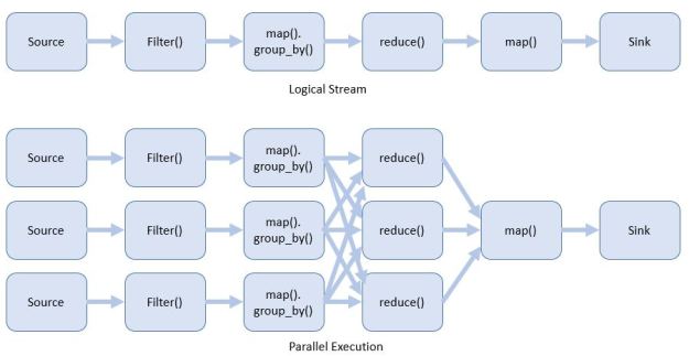
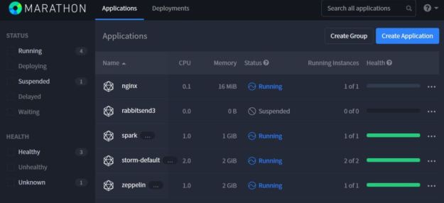
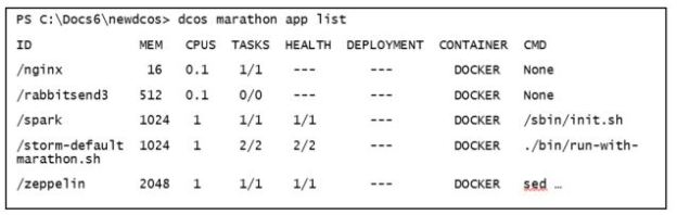
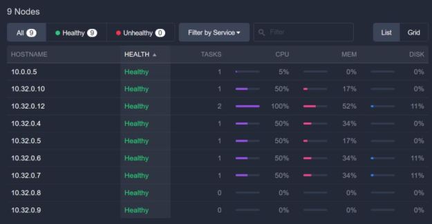
Figure 1.  DCOS web interface.

DCOS is the distributed cluster operating system and its job is to support deployed services.   The most valuable of these services is Marathon which is a container orchestration service that will allow you to easily scale the number instances of your containers and keep them running.   It can also be used to enforce special constraints.   For example, if you deploy a docker container that needs to bind to a special port on they host, it will not schedule another conflicting instance on that same host.   And it has a very nice graphical user interface shown in figure 2 that can be accessed through the DCOS interface.

dcos2

Figure 2.   Marathon interface showing all running services.

As you can see above I have an instance of Apache Spark, two instances of the streaming service Storm and one instance of the Zeppelin notebook and one instance of the simple web server Nginx all running.  Launching a new Docker container or service is very simple: fill in a web-form.    However, there is a command line tool that works very well on linux and windows.  For example, to get the information in Figure 2 above the command line call is as follows.

dcos7

The same command line interface can be used to launch new container instances and we will illustrate that below.

DCOS also has views of the of the individual resources.   Figure 3 displays the current view of all of the individual nodes in the cluster showing how many of the nodes are holding active containers or services.

dcos3

Figure 3.  DCOS display of worker node status and load

A Simple Example.

There are many prepackaged apps available for a one-click launch such as those listed above.  I originally wanted to Kafka in a demo, but there is still a bug with my deployment that does not allow me to access the Kafka gateway or the public node (10.0.0.5 in the Figure 3 list).   I will revise this report with an update as soon as I can solve that problem.

The example is a simple message filtering experiment.   Assume you have some source of independent tasks that must be analyzed as fast as possible and the results stored in a table or database.  Assume further that you task stream can be pre-filtered into and sorted into buckets of similar tasks that can be analyzed by code that is best suited for the tasks in that bucket.  For example, some tasks contain images of landscapes and others contain images of animals and you want to provide analyzers that are appropriate for each.   Or you are looking at logging data and your pre-filters detect several different types of anomalies and you want to group anomalies of similar type together.   We will use queues to hold the contents of each bucket.  The pre-filters push the data into the queues and workers pull the tasks of the queue, do the analysis and push the results to into a table. The general picture is shown in Figure 4 below.

dcos4

Figure 4.   Sample “microservice” configuration for our experiment.

Depending upon the complexity of the analysis undertaken by the worker and the arrival rate of tasks into the queues we may need to increase the number of workers assigned to each bucket queue as shown in Figure 5.

dcos5

Figure 5.   Adding additional workers to manage extra work at each queue.

In this simple experiment we will look at how increasing the number of workers can improve the throughput of the system.   Now for the details of the set-up.   Instead of using Kafka, we will use another common message broker RabbitMQ that is running on another linux box on Azure.   We use the Azure Table service to store the results.   Our worker service is a Docker container that is running a simple Python program that has two parts.

  1. When the worker starts-up it does not know what queue to list to.    So it looks in a separate queue called “roles” that will contain the name of the queue needed an extra worker.
  2. When it has the name of the queue to work on and begin pulling data items from the given queue and processing them and saving them to the table.  A time stamp is added to each item as it goes into the table.

In a real application step 2 can include task specialization once the worker knows what queue it is working on.  For example, in our text classifier example we loaded specific machine learning tables and states when we knew what topics we were analyzing.

In this example, we are only interested in the basic scale-up performance improvement as we increase the number of workers assigned to each queue.    The Python code for the container is not pretty, but you  are welcome to read and use it.   It is on GitHub here.   To deploy the Docker container on DCOS one needs a deployment configuration json file.  This config.json is shown below.

{
   "container": {
      "type": "DOCKER",
      "docker": {
          "image": "escigrp/rabbitpullpush"
       }
    },
   "id": "worker",
   "instances": 1,
   "cpus": 0.2,
   "mem": 512,
}

Notice that this specifies that the container is in the Docker hub with the name escigrp/rabbitpullpush and that we wish to devote 0.2 cpus and 512 MB of memory to this resource.  And we want one instance.

The dcos command to launch this container in the cluster is

dcos marathon app add config.json

Our “worker” will immediately show up as a deployment on the DCOS Marathon web page.

We are going to measure the throughput of the system in the number of events per second it can process as we increase the number of workers per node.   The way the experiment is done is as follows

For N = 1 to 14:

  1. Preload each of the 4 queues (named “1”, “2”, “3”, “4”) with 500 messages and start up 4*N instances of the worker container with Marathon on DCOS.
  2. Load the “roles” queue with N instances of each queue name.   Each of the four queues will now have N devoted workers.
  3. When all of the queues are empty, look in the table.   Subtract the earliest time stamp from the latest to get an approximation of the elapsed time.
  4. Use marathon to shutdown the workers and go to step 1.

Recall that there are 8  dual core nodes in the cluster.   Each instance of the worker container is allocated 0.2 of a core.   This means marathon could possibly schedule 80 instances.   However, there are other processes running on cluster so a practical limit was 60.   In fact we tested up to 56 container instances (14*4).   The results are shown in Figure 6 below.

dcos6

Figure 6.   Events processed per second as the number of workers per queue grows from 1 to 14.

There are several surprises for me here.   First the performance scales very linearly as the number of container instances grows.   Because there are only 16 cores available I expected this to level off when N was near 8  (32 instances), but, with the exception of an anomaly around 13, it kept climbing to N = 14 (56 instances).    Second, the absolute performance is not very good.   Digging deeper into the code and conducting several additional experiments revealed that the bottleneck is the table insertion due to an old and slow version of the python library.  Without the table insertion a single worker container instance call pull events at a rate of about 20 events per second, so 56 instances will be over 1000 events/sec which is well within the range of RabbitMQ.

Dynamic Scaling and Conclusion

A more interesting experiment would be to have the system described above dynamically scale the number of container instances as circumstances require.   For example, if one could monitor the depth of each queue, then if a queue starts to grow larger one could issue a command to increase the number of instances devoted to that queue.  If the queue is empty one could reduce the number of instances.    I am fairly certain there are a number of ways to do this, but one easy way is to use the “marathon update” command.   This command allows a “real-time” update to json configuration.    Any field in the configuration can be modified.   For example, to  update the configuration to 10 instances one can issue the command below.

dcos marathon app update worker env='{"instances":"10"}'

This change in status should trigger marathon to make the necessary adjustments and change the number of instances to 10.   It would be relatively straight forward to write a program that would poll the event broker for status and check the current queue lengths and, depending on the conditions issue the dcos command above.

Final Thoughts.

It is great to see this container service based on Mesosphere’s DC/OS finally available in a reliable and highly usable form.   This an excellent platform for managing large collections of Docker containers and orchestrating microservices deployments.   The performance of the system was excellent and the web user interface is well done.   The command line interface is solid and only gave me one problem.   Installing the command line interface for Kafka caused problems on windows and it did not follow the script here.  It seemed to be loading an old version that did not support windows.   The other problem was that the DC/OS cluster I deployed on Azure had one public node, but the “public” IP address give for this node was not reachable.   (Any reader who knows how to address these problems please comment here and I will update this post.  As is often the case, there are easy solutions to problems that stump me.)

In a future post we will look at the Docker Swarm deployment that is also part of this new Azure release.

Fun with Recurrent Neural Nets: One More Dive into CNTK and TensorFlow

In a previous article I set about comparing Microsoft’s Computational Network Took Kit for deep neural nets to Google’s TensorFlow.  I concluded that piece with a deep dive into how recurrent neural nets (RNNs) were represented in each system.   I specifically went after the type of RNNs known by the strange name of Long Short-Term Memory (LSTM) networks.   I wanted to learn a bit more about how these systems worked.  I decided to treat them like laboratory specimens so that I could poke and prod them to see what I could learn and what I could get them to do.  This article is essentially my lab notebook.  Warning:  With the exception of a bit toward the end, this is not technically very deep.   In fact, I did not discover anything that has not been extensively reported on elsewhere.   But I learned a lot and had some fun.   Perhaps it will be of interest to students just starting to learn about this subject.   Before I get to far into this, I would like to mention that I recently discovered an excellent series of tutorials on RNNs by Denny Britz that are definitely worth reading.

CNTK’s LSTM and Hallucinating Bloomberg Financial News

One of the many good examples in CNTK is language modeling exercise in Examples/Text/PennTreebank.   The documentation for this one is a bit sparse and the example is really just of a demo for how easy it is to use their “Simple Network Builder” to define a LSTM network and train it with stochastic gradient decent on data from the Penn Treebank Project.   One command starts the learning:

cntk configFile=../Config/rnn.cntk

Doing so trains the network, tests it and saves the model.  However, to see the model data in an easily readable form you need a trivial addition to the configfile: you need to add the following dumpnode command to put a dump file a directory of your choosing.

dumpnode=[
    action = "dumpnode"
    modelPath = "$ModelDir$/rnn.dnn"
    outputFile = "$OutputDir$/modeltext/dump"
]

This creates a big text file with all the trained data.   To experiment with the trained model, I decided to load it into a python notebook and rebuild the LSTM network from the defining equations.  From the CNTK book those equations are

lstm_eqn

I was pleased to see that the dumped model text had the same W and b tensors names as in the equations, so my job was relatively easy.    I extracted each of the tensors and saved them into a file (I will make these available in Github).   The python code for the LSTM based on the equations above is below.

def rnn(word, old_h, old_c):
      Xvec = getvec(word, E)

      i = Sigmoid(np.matmul(WXI, Xvec) + 
                  np.matmul(WHI, old_h) + WCI*old_c + bI)
      f = Sigmoid(np.matmul(WXF, Xvec) + 
                  np.matmul(WHF, old_h) + WCF*old_c + bF)
      
      c = f*old_c + i*(np.tanh(np.matmul(WXC, Xvec) + 
                               np.matmul(WHC, old_h) + bC))
      
      o = Sigmoid(np.matmul(WXO, Xvec)+ 
                  np.matmul(WHO, old_h)+ (WCO * c)+ bO)
      
      h = o * np.tanh(c)
      
      #extract ordered list of five best possible next words
      q = h.copy()
      q.shape = (1, 200)
      output = np.matmul(q, W2)
      outlist = getwordsfromoutput(output)
      return h, c, outlist

As you can see, this is almost a literal translation of the equations.    The only different is that this has as input a text string for the input word.  However the input to the equations is a vector encoding of the word.  The model generates the encoding matrix E which has the nice property that the ith column of matrix corresponds to the word in the ith position in the vocabulary list.  The function getvec(word, E) takes the embedding tensor E, and looks up the position of the word  in the vocabulary list and returns the column vector of E that corresponds to that word.   The output of one pass through the LSTM cell is the vector h.  This is a compact representation of the words likely to follow the input text to this point.  To convert this back into “vocabulary” space we multiply it by another trained vector W2.  The size of our vocabulary is 10000 and the vector output is that length.  The ith element of output represents the relative likelihood that that ith word is next word to follow the input so far.  Getwordsfromoutput simply returns the top 5 candidate words in order of likelihood.

Before going further, it is worth looking closer at the properties of the word embedding matrices E and W2.   There is a fascinating paper by  Mikolov, Yih and Zweig entitled “Linguistic Regularities in Continuous Space Word Representations” where they suggest that the embedding space for word has several interesting properties.   I decided to investigate that.   Their point is that words that are similar in a linguistic sense will be nearby in the embedding space.   For example, present tense verbs should be near other present tense verbs and singular nouns should be near each other, etc.   I decided to try that.  However, there are two embedding mappings.  One is based on the tensor E and the other based on the W2 tensor.   E has dimension 150 by 10000 and W2 is 200 by 10000.  The difference in dimensionality are because of arbitrary decisions made in defining the hidden layers in the network.  But both represent word imbeddings.  I experimented with both.  I wrote a function getnear(word, M) which takes a word and looks for the 5 most nearby words in the space where M is transpose of either E or W2. (I used cosine distance as the metric.) Verb tense locality and noun plurals worked best in the W2 space as illustrated below.

rnn-embedding

These are only illustrations.  For a deeper statistical analysis look at the Mikolov paper.   A more interesting conjecture from their study was that there may be some linearity in these embedding that might allow one to try simple analogies of the form “A is to B, as C is to __”.   Their idea is that if a, b and c are the vector embeddings of the words A, B and C, then the embedding of “__” may be computed as d = c + (b-a).  So I wrote a little function AistoBasCisto(A, B, C) that does this computation.   In the results I had to delete A, B and C from the candidate answers because they came up often as nearby.   In this case my results were less encouraging.  It worked better with the E space than with W2.   For example, for E we have

rnn-analogy1

And for the W2 space the results looked like

rnn-analogy2

As you can see the “run running walk __” example failed with E but was close, but still incorrect, with W2.

You may wonder why these particular words came up.  The data we used to train the system came from a small subset of the Penn TreeBank collection as provided in the CNTK package.   It is heavily dominated by financial news items.    This explains why the plural of person could be managers or customers.   A larger vocabulary and data collection would be needed to truly test the analogy by linearity conjecture.

Now on to hallucinating the financial news.

Now to test the LSTM as a truly recurrent network.   We provide the network with a starting word and let it suggest the next word.  And then we repeat this process constructing a “sentence”.  In the code below we randomly pick one of the top three suggest by the network as the next word.

c = np.zeros(shape = (200, 1))
h = np.zeros(shape = (200, 1))
output = np.zeros(shape = (10000, 1))
word = 'my'
sentence= word 
for _ in range(40):
    h, c, outlist = rnn(word, h, c)
    word = outlist[randint(0,3)]
    sentence = sentence + " " +word
print sentence+"."

In this case we start with the word “my” and let it generate a 40 word sentence.  The output is

my new rules which would create an interest position here unless there should prove   signs of such things too quickly although the market could be done better toward paying further volatility where it would pay cash around again if everybody can.

This is a great example of hallucinating financial news. Let’s try it again starting with the word “president”.

president michael de brown wrote himself against democratic union law which represents an emergency relief agreement during a new york state district or early tuesday before july after a federal government agency created early losses without mr. krenz or perhaps.

Now with the word “the”.

the company reported third-quarter results reflecting a number compared between N barrels including pretax operating loss from a month following fiscal month ending july earlier compared slightly higher while six-month cds increased sharply tuesday after an after-tax loss reflecting a strong.

The “sentences” end rather abruptly because of the 40 word limit I set.  If you let it go it will run on until the state vector for the sentence seems to break down.     Try this yourself.  To make it easy to play with this example, I have put the code in GitHub.  The trained model text files are in OneDrive and is a zipped file of about 50MB.

There are many more excellent and fun examples.  Andrej Karpathy has a great blog article showing how RNNs can mimic Shakespeare, or Latex science articles and many more.

TensorFlow’s seq2seq French Lesson.

One of the most interesting examples in the TensorFlow tutorials is an English to French translator.  As with the CNTK example it was trivial to start the translator learning following the instructions in the tutorial.   After letting this run for about a week, I wanted to see how well it would do.     As with the CNTK example, I created a Jupyter IPython notebook and loaded the trained model.   I will explain how that was done in more detail below but, for now, I will show how we can invoke it to test its translation ability.    This particular trained model was not very big and with a relatively small data set, so I didn’t expect much.    In fact, as you will see, to a French speaker it is a disaster.   On the other hand, it learned more French in a week of training that I did in three semesters of French in college.   (For full disclosure, this was my weakest subject in college and my grade was a hard-fought “C” each semester.)

The code below demonstrates how the model is invoked.   First you have to tokenize the input sentence.  The algorithm uses a system of buckets of fixed sizes to make the training more efficient.  You next find the smallest bucket that can contain your sentence and convert this to the input vector list needed by the model.   The step function takes a Tensorflow session, the input vector list and a null list of decoder inputs (to be explained later) and generates a list of vectors as outputs.  Each vector represents the likelihood that individual vocabulary words are the correct word at that point in the translated sentence.   We pick the most likely and print the sentence.

sentence = " I am not the president of France. "

token_ids = data_utils.sentence_to_token_ids(sentence, en_vocab)
      # Which bucket does it belong to?
bucket_id = min([b for b in xrange(len(_buckets))
                 if _buckets[b][0] > len(token_ids)])
      # Get a 1-element batch to feed the sentence to the model.
encoder_inputs, decoder_inputs, target_weights = 
    model.get_batch({bucket_id: [(token_ids, [])]}, bucket_id)

_, _, output_logits = model.step(sess, encoder_inputs, decoder_inputs, 
                                 target_weights, bucket_id, True)
		  
outputs = [int(np.argmax(logit, axis=1)) for logit in output_logits]
print(" ".join([rev_fr_vocab[output] for output in outputs]))

Je ne suis pas le président de la France .

This example is not too bad.  However, if I ask

“In which city does the president of France live?”

I get

“Dans quelle ville le président de la France ?”.

This is not exactly correct.    If I feed this into Google translate and ask what this means in English I get “In which city the President of France?”.   If I give it this one,

What is the name of a good restaurant?

The system responds with

Quel est le nom d’une bonne bonne bonne ?”

Which translates back to “What is the name of a good good good?”.  Probably not very helpful on the streets of Paris.   It turns out restaurant is not in the tiny training vocabulary used here.   Finally, given this sentence

” The article stated that the President of the United States is here today. “

The translator returned

Le paragraphe a indiqué que le président des États-Unis est aujourd ‘ hui aujourd ‘ hui .”

The end of this reply is “is today today”.    As I said, this is still much better than I could do with my college French.   However, as you can see from the previous two examples, our little translator runs out of gas at the end of sentences and tends to repeat itself.   You should try this yourself.   I have put the notebook file in github or you can execute these directly from the Tensorflow python code.   All you need to do is train the model from TensorFlow and run the notebook with the path to the model output directory.

While loading and using the trained model was easy and fun, understanding the seq2seq model used in this example takes a bit of work.   So this part of this article will get a bit more technical.

The TensorFlow translate program is based on a sequence-to-sequence model constructed from more primitive recurrent neural nets.   By sequence-to-sequence we mean a network that takes a sequence as input and produces a sequence as output.   It consists of two parts: an “encoder RNN” and a “decoder RNN” as shown in Figure 1 below.

seq2seq

Figure 1.   A sequence-to-sequence RNN English to French translator with the encoder and decoder unrolled to show the flow of messages.

In this figure the RNNs are “unrolled” to show the flow of messages.  The state vector at the end of the encoder is a vector embedding of the input sentence.   This state vector is used to start the decoder along with a “GO” token.  The diagram shows the network after it has been trained.   During training the inputs to the decoder are the French version of the English sentences.   I won’t talk about the training here because is enough to try to understand how this works.  Before I go any further I want to point you to some important papers.  Sutskever, Vinyals and Le published an early important paper on sequence to sequence models that is worth reading.

To understand how it is built the network we need to dig into the code a bit. The building blocks are a set of classes of base type RNNCell with specializations

  1. BasicRNNCell
  2. GRUCell
  3. BasicLSTMCell
  4. LSTMCell
  5. OutputProjectionWrapper
  6. InputProjectionWrapper
  7. EmbeddingWrapper
  8. MultiRNNCell

The ones we will see used here are GRUCell, MultiRNNCell and EmbeddingWrapper.   We discussed LSTMCell in our previous article but we need to look at GRUCell here because that is the one used in the example.   The GRUCell is a “Gated Recurrent Unit” invented by Cho et. al.  in “Learning Phrase Representations using RNN Encoder–Decoder for Statistical Machine Translation”.  The “gated” phrase comes from the way the output is defined as coming mostly from the previous state or from a combination with the new input.   The diagram below tries to explain this a bit better.

gru-pic

Figure 2.   GRU wiring diagram

It also helps to see it in terms of the defining equations.

gru-eq1

The quantity ut  is a gate vector.  Recall the sigmoid function switches sharply between one and zero.  So when ut is one then h is just a copy of the old h and we are ignoring the input x it is based on the value ct.   The gate rt is determines how much of the old state goes into defining the value of ct.   To understand how this is encoded in TensorFlow you need to understand the function.

linear(args, output_size, bias, bias_start=0.0, scope=None)

where args is a list of tensors each of size batch x n .   Linear computes sum_i(args[i] * W[i]) + bias where W is a list of matrix variables of size n x outputsize and bias is a variable of size outputsize.   In the equations above we have represented linear algebra as a matrix times a column vector.   Tensorflow uses the transpose notation:   row vector on the left times the transpose of the matrix.   So in linear the args are a list of row vectors.   Where is the matrix W and offset b?  This is fetched from memory based on the variable current scope, because W and b are variable tensors that are learned values.   If you look at the first two equations above, you will see they are almost identical.   In fact, we can write them as

gru-eq2

If you transpose the last one from column form into row form you can now compute both with one invocation of the linear function.   The code for the GRUCell is below.   As you can see they have encoded one pass through the GRU cell with only two matrix vector multiplies.   You can also see that the way the variable scope is used to pick out the W’s for the gates and the W for the state/output.  Another point to remember that an invocation of the “__call__ function operator does not cause the tensor to execute the operation, rather it builds the graph.

class GRUCell(RNNCell):
  def __init__(self, num_units):
    self._num_units = num_units
   ... stuff deleted ....
  def __call__(self, inputs, state, scope=None):
    with vs.variable_scope(scope or type(self).__name__):  
      with vs.variable_scope("Gates"):  # Reset gate and update gate.
        # We start with bias of 1.0 to not reset and not udpate.
        r, u = array_ops.split(1, 2, linear([inputs, state],  
                               2 * self._num_units, True, 1.0))
        r, u = sigmoid(r), sigmoid(u)
      with vs.variable_scope("Candidate"):
        c = tanh(linear([inputs, r * state], self._num_units, True))
      new_h = u * state + (1 - u) * c
    return new_h, new_h

The top level class we invoke for building our model is seq2seqModel.    When we create an instance of this class it sets in motion a set of flowgraph building steps.  I am going to skip over a lot of stuff and try to give you the big picture.  The first graph building step in the initialization of an instance of this object is

# Create the internal multi-layer cell for our RNN.
    single_cell = rnn_cell.GRUCell(size)
     …
    if num_layers > 1:
      cell = rnn_cell.MultiRNNCell([single_cell] * num_layers)

As you can see we are creating a GRU cell graph generator instance and making a list of num_layers of this object and passing that to the constructor for MultiRNNCell.   In our case, num_layers has been set to 2.   MultiRNNCell is pretty easy to understand.   It builds a graph consisting of a stack of (in this case) GRU cells where the output state vector of each level is fed to the input of the level above it.  This new compound cell has an output that is the state of the top sub-cell and whose output state is the concatenation of the output states of all the sub-cells.

The next part is not so easy to follow.    We will take our MultiRNNCell graph builder and use it to create and encoder and a special decoder.    But first we must make a short digression.

Paying Attention

There is a problem that is encountered in the sequence-to-sequence model.   The encoder encodes the entire sentence into a state vector which is used by the decoder as its input.    That state vector is an abstract representation of our entire sentence as a single point in a very high dimensional space.    The decoder has been trained to use that point as a starting point to unroll a translated version of the sentence.   I find the fact that it works at all to be rather remarkable.   It is as if the decoder takes the English state vector and transforms it into a similar point in “French” space.

Unfortunately, the longer the input sentence, the more difficult it is to decode it.   How much information can we pack into one point?   The problem is that at each decoding step we need a little bit more information than is provided by the state vector as it passes through the decoder loop.   The idea used here is to help the decoder by providing it a bit of focus derived from the input sequence at each stage of the decoder loop.  This is generally referred to as “attention”, as in “at this step of decoding please pay attention to what the encoder was doing here”.   Bahdanau, Cho and Bengio had an early paper about this that used a bidirectional pass over the input sequence. As they put it, they wanted to “automatically (soft-)search for parts of a source sentence that are relevant to predicting a target word”.  (Denny Britz has a lovely blog article about attention and describes several fascinating applications.  It is  well worth  reading.) The mechanism for attention used in the TensorFlow example is based on a paper by Vinyals et. al. and we will follow that one here.   The key idea is rather than take the single final state vector from the encoder, let’s collect the state vectors at each stage of the encoder.   Following Vinyals, let the encoder state vectors for each input word be

atten1

And let the decoder state vectors be

atten2

Then for each decoder time step t compute

atten3

Where the Ws are learned matrices and v is a learned vector.    Then as the input to the t+1 state vector of the decoder we use the concatenation

atten4

The idea is this new state vector at time t+1 puts much more focus on the corresponding words in in the encoder string. This all happens in a function called seq2seq.attention_decoder that is called in another constructor function seq2seq.embedding_attention_seq2seq that wraps and an embedding around a graph generated by our MultiCellRNN graph builder to generate the final decoder graph.   These graphs are all stitched together in the Seq2SeqModel constructor.  It is fair to say that there are many levels of abstraction here that are used to build the decoder and link it to the encoder.  I am leaving out many details that are critical for the training such as the part that implements the bucket handler.   The final graph, in its most abstract form is pictured below in figure 3.

seq2seq_final

Figure 3.  The Translate.py sequence to sequence translator is based on a two level GRU cell encoder and an attention-augmented two level GRU cell decoder.  The input English is entered in reverse order as an optimization

Final Thoughts

As I have said above, I have not included all the details of how the seq2seq translator is put together, but I tried to include the highlights that I found most interesting.   I encourage you to dive into the code and discover the rest.   You will likely find some errors in what I described above.   If so, please let me know.

There is really a lot of exciting results that have come out in the last few years relating to RNNs.   For example, Lei Ba, Mnih and Kavukcuoglu demonstrated that RNNs with attention can be applied to interesting image analysis challenges, such as reading the house number from a street scene.   In “Teaching Machines to Read and Comprehend” Hermann et. al. excellent paper demonstrate the use of an attentive RNN build to answer simple questions about text.   I personally don’t think any RNN can pass a Turing test yet, so it ain’t A.I.  But these little statistical machines are certainly wonderful mimics and they can speak better French than I.

TensorFlow Meets Microsoft’s CNTK

Updated April 4, 1017.   Much of this material has been updated and improved and now appears as Chapter 10, Cloud Computing for Science and Engineering.  It can be accessed at the book’s website.

Update Nov 10, 2016.   Microsoft now has  a new release of CNTK.  We have a post now that provides a quick look at this new version.  Go read that one instead of this one.

Update Oct 25, 2016.    this post describes the early version of CNTK.  Microsoft just released a very nice new version called the cognitive toolkit.   I would not base your impression of CNTK  on the following post.   I’ll update this as soon as I have time.

———————–

CNTK is Microsoft’s Computational Network Toolkit for building deep neural networks and it is now available as open source on Github.   Because I recently wrote about TensorFlow I thought it would be interesting to study the similarities and differences between these two systems.   After all, CNTK seems to be the reigning champ of many of the image recognition challenges.   To be complete I should also look at Theano, Torch and Caffe.   These three are also extremely impressive frameworks.   While this study will focus on CNTK and TensorFlow I will try to return to the others in the future.   Kenneth Tran has a very nice top level (but admittedly subjective) analysis of all five deep learning tool kits here.  This will not be a tutorial about CNTK or Tensorflow.  Rather my goal is to give a high level feel for how they compare from the programmer’s perspective.  This is not a performance analysis, but rather a programming model analysis.  There is a lot of code here, so if you don’t like reading code, skip to the conclusions.

CNTK has a highly optimized runtime system for training and testing neural networks that are constructed as abstract computational graphs.   In that sense, CNTK is very much like TensorFlow.   However, there are some fundamental differences.   To illustrate these features and differences I will take two standard examples that are included with both systems and work through the approach taken by each system.   The first example is a not-too-deep convolutional neural net solution to the standard MNIST handwritten digit recognition example.  I will conclude with some comments about how they differ in their approach in the case of recurrent neural networks.

Both TensorFlow and CNTK are basically script-driven.   By this I mean that the construction of the neural network flow graph is described in a script and the training is done using some very clever automated processes.   In the case of TensorFlow the script is embedded in the Python language and Python operators can be used to control the flow of execution of the computational graph.   CNTK does not currently have a Python or C++ binding (though one is promised) so currently the control flow of the execution of the training and testing is highly choreographed.    As I will show, this is not as much of a limitation as it sounds.   There are actually two scripts associated with a CNTK network:  a configuration file that controls the training and test parameters and a network definition language file for constructing the network.

I’ll start with the description of the neural network flow graph because that is where the similarity to TensorFlow is the greatest.   There are two ways to define the network in CNTK.  One approach is to use the “Simple Network Builder” that will allow you to create some simple standard networks by specifying only a few parameter settings.    The other is to use their Network Definition Language (NDL).   The example here (taken directly from their download package in Github) uses NDL.    Below is a slightly abbreviated version of the Convolution.ndl file. (I have used commas to put multiple lines on one line to fit the page better.)

CNTK network graphs have a set of special nodes.  These are FeatureNodes and LabelNodes that describe the inputs and training labels,  CriterionNodes and EvalNodes that that are used for training and result evaluation, and OutputNodes that represent the outputs of the network.   I will describe these below as we encounter them.   At the top of the file we have a set of macros that are used to load the data (features) and labels.   As can be seen below we read images of the MNIST digits as features which are now arrays of floating point numbers that we have scaled by a small scalar constant.   The resulting array “featScaled” will be used as input to the network.

load = ndlMnistMacros

# the actual NDL that defines the network
run = DNN

ndlMnistMacros = [
    imageW = 28, imageH = 28
    labelDim = 10

    features = ImageInput(imageW, imageH, 1)
    featScale = Const(0.00390625)
    featScaled = Scale(featScale, features)
    labels = Input(labelDim)
]

DNN=[
    # conv1
    kW1 = 5, kH1 = 5
    cMap1 = 16
    hStride1 = 1, vStride1 = 1
    conv1_act = ConvReLULayer(featScaled,cMap1,25,kW1,kH1,hStride1,vStride1,10, 1)

    # pool1
    pool1W = 2, pool1H = 2
    pool1hStride = 2, pool1vStride = 2
    pool1 = MaxPooling(conv1_act, pool1W, pool1H, pool1hStride, pool1vStride)

    # conv2
    kW2 = 5, kH2 = 5
    cMap2 = 32
    hStride2 = 1, vStride2 = 1
    conv2_act = ConvReLULayer(pool1,cMap2,400,kW2, kH2, hStride2, vStride2,10, 1)

    # pool2
    pool2W = 2, pool2H = 2
    pool2hStride = 2,  pool2vStride = 2
    pool2 = MaxPooling(conv2_act, pool2W, pool2H, pool2hStride, pool2vStride)

    h1Dim = 128
    h1 = DNNSigmoidLayer(512, h1Dim, pool2, 1)
    ol = DNNLayer(h1Dim, labelDim, h1, 1)

    ce = CrossEntropyWithSoftmax(labels, ol)
    err = ErrorPrediction(labels, ol)

    # Special Nodes
    FeatureNodes = (features)
    LabelNodes = (labels)
    CriterionNodes = (ce)
    EvalNodes = (err)
    OutputNodes = (ol)
]

The network is defined in the block DNN.   The network consists of two convolutional-maxpooling layers followed by an all-to-all standard network with one hidden later of 128 nodes.

In convolutional layer one we have 5×5 convolutional kernels and we specify 16 of these (cMap1) for the parameter space.   The operator ConvReLULayer is actually a shorthand for another subnetwork defined in a macro file.

Algebraically we would like to represent the parameters of the convolution as a matrix W and a scale vector B so that if the input is X, the output of our network layer is of the form output = f(op(W, X) + B).   In this case the operator op is convolution and f is the standard relu function relu(x)=max(x,0).

The NDL code for the ConvReLULayer is given by

ConvReLULayer(inp, outMap, inWCount, kW, kH, hStride, vStride, wScale, bValue) = 
[
    convW = Parameter(outMap, inWCount, init="uniform", initValueScale=wScale)
    convB = Parameter(outMap, 1,        init="fixedValue", value=bValue)
    conv = Convolution(convW, inp, kW, kH, outMap, hStride,vStride,
                zeroPadding=false)
    convPlusB = Plus(conv, convB);
    act = RectifiedLinear(convPlusB);
]

The W matrix and B vector are defined as Parameters and they will be the entities that are given an initial value and then modified during training to define the final model.   In this case convW is a matrix with 16 rows of 25 columns B is a scale vector of length 16.   Convolution is a built-in function that has been set to not use zero padding.  This means that convolution over the 28×28 image will be centered on the 24 by 24 interior region and the result will be 16 variations of a 24×24 output sudo-image.

We next apply Maxpooling based on 2×2 regions and the result is now 12×12 by 16.

convo-nn-cntk

For the second convolutional layer we up the number of convolutional filters from 16 to 32.  This time we have 16 channels of input so the size of the W matrix is 32 rows  of 25×16 = 400 and the B vector for this layer is 32 long.   The convolution is now over the interior of the 12×12 frames so it is size 8×8 and we have 32 copies.    The second maxpooling step takes us to 32 frames of 4×4 or a result of size 32*16 = 512.

The final layers have the 512 maxpooling output and a hidden layer of 128 nodes to a final 10 node output defined by the two operators

DNNSigmoidLayer(inDim, outDim, x, parmScale) = [
    W = Parameter(outDim, inDim, init="uniform", initValueScale=parmScale)
    b = Parameter(outDim, 1,     init="uniform", initValueScale=parmScale)
    t = Times(W, x)
    z = Plus(t, b)
    y = Sigmoid(z)
]

DNNLayer(inDim, outDim, x, parmScale) = [
    W = Parameter(outDim, inDim, init="uniform", initValueScale=parmScale)
    b = Parameter(outDim, 1,     init="uniform", initValueScale=parmScale)
    t = Times(W, x)
    z = Plus(t, b)
]

As you can see these are defined by the standard linear algebra operators as W*x+b.

The final part of the graph definition is the cross entropy and error nodes followed by a binding of these to the special node names.

We will define the training process soon, but first it is fun to compare this to the construction of a very similar network in TensorFlow.   We described this in a previous post but here it is again.   Notice that we have the same set of variables as we did with CNTK except they are called variables here and parameters in CNTK.   The  dimensions are also slightly different.  The convolutional filters 5×5 in both cases but we have 16 copies in the first stage and 32 in the second in CNTK and 32 in stage one and 64 in stage two in the TensorFlow example.

def weight_variable(shape, names):
  initial = tf.truncated_normal(shape, stddev=0.1)
  return tf.Variable(initial, name=names)

def bias_variable(shape, names):
  initial = tf.constant(0.1, shape=shape)
  return tf.Variable(initial, name=names)

x = tf.placeholder(tf.float32, [None, 784], name="x")

sess = tf.InteractiveSession()

W_conv1 = weight_variable([5, 5, 1, 32], "wconv")
b_conv1 = bias_variable([32], "bconv")
W_conv2 = weight_variable([5, 5, 32, 64], "wconv2")
b_conv2 = bias_variable([64], "bconv2")
W_fc1 = weight_variable([7 * 7 * 64, 1024], "wfc1")
b_fc1 = bias_variable([1024], "bfcl")
W_fc2 = weight_variable([1024, 10], "wfc2")
b_fc2 = bias_variable([10], "bfc2")

The network construction is also almost identical.

def conv2d(x, W):
  return tf.nn.conv2d(x, W, strides=[1, 1, 1, 1], padding='SAME')

def max_pool_2x2(x):
  return tf.nn.max_pool(x, ksize=[1, 2, 2, 1],
                        strides=[1, 2, 2, 1], padding='SAME')

#first convolutional layer
x_image = tf.reshape(x, [-1,28,28,1])
h_conv1 = tf.nn.relu(conv2d(x_image, W_conv1) + b_conv1)
h_pool1 = max_pool_2x2(h_conv1)
#second convolutional layer
h_conv2 = tf.nn.relu(conv2d(h_pool1, W_conv2) + b_conv2)
h_pool2 = max_pool_2x2(h_conv2)
#final layer
h_pool2_flat = tf.reshape(h_pool2, [-1, 7*7*64])
h_fc1 = tf.nn.relu(tf.matmul(h_pool2_flat, W_fc1) + b_fc1)
h_fc1_drop = tf.nn.dropout(h_fc1, keep_prob)
y_conv=tf.nn.softmax(tf.matmul(h_fc1_drop, W_fc2) + b_fc2)

The only differences are that the convolutional operators here are defined with padding so the output of the first convolutional operator had dimensions of 28 by 28 flowed by a pooling reduction to 14 by 14.  The second convolutional operator and max pooling reduces this to 7×7, so the input to the final layer is 7x7x64 = 3136 with 1024 hidden nodes (with a relu instead of a sigmoid function).   (For training purposes the last stage uses a probabilistic dropout function that randomly set values to zero.   If keep_prob = 1, this is a no-op. )

convolutional

Network Training

The way network training is specified in CNTK differs substantially from the TensorFlow approach.  The training and testing is specified in a file called convolution.config.  Both CNTK and TensorFlow use a symbolic analysis of the flow graph to compute the gradient of the network for use in gradient decent training algorithms.  The CNTK team has a very nice “book” that describes a great deal about how the gradients are computed.   Currently CNTK only supports one learning method: Mini-batch Stochastic Gradient Decent, but they promise to add more in the future.  He, Zhang, Ren and Sun have a lovely paper that describes how they train extremely deep (up to 1000 layers) networks using a nested residual reduction method reminiscent of algebraic multi-grid, so it will be interesting to see if that method makes its way into CNTK.  An abbreviated version of the config file is shown below.

command = train:test
modelPath = "$ModelDir$/02_Convolution"
ndlMacros = "$ConfigDir$/Macros.ndl"

train = [
    action = "train"
    NDLNetworkBuilder = [
        networkDescription = "$ConfigDir$/02_Convolution.ndl"
    ]

    SGD = [
        epochSize = 60000
        minibatchSize = 32
        learningRatesPerMB = 0.5
        momentumPerMB = 0*10:0.7
        maxEpochs = 15
    ]

    reader = [
        readerType = "UCIFastReader"
        file = "$DataDir$/Train-28x28.txt"

        features = [
            dim = 784
            start = 1
        ]

        labels = [
		    # details deleted
        ]
    ]
]
test = [
   ….
]

The command line indicates the sequence to follow:  train then test.   Various file paths are resolved and then the train block specifies the network to be trained and the parameters for the Stochastic Gradient Decent (SGD).  A reader block specifies the way the “features” and “labels” from the network NDL file are read.   A test block is also included to define the parameters of the test.

Running this on a 16-core (non-GPU) linux VM took 62.95 real-time minutes to do the train and test and 999.01 minutes of user time and 4 minutes of system time.    The user time indicated that all 16 cores were all very busy (999/63 = 15.85).   Of course this means little as CNTK is designed for parallelism and massive GPU support is the true design point idea.

The training used by TensorFlow is specified much more explicitly in the Python control flow.   However, the algorithm is also a gradient based method called Adam introduced by Kingma and Ba.    Tensorflow has a number of gradient based optimizers in the library, but I did not try any of the others.

As can be seen below, the cross_entropy is defined in the standard way and fed to the optimizer to produce a “train_step” object.

y_ = tf.placeholder(tf.float32, [None, 10])
cross_entropy = -tf.reduce_sum(y_*tf.log(y_conv))
train_step = tf.train.AdamOptimizer(1e-4).minimize(cross_entropy)
correct_prediction = tf.equal(tf.argmax(y_conv,1), tf.argmax(y_,1))
accuracy = tf.reduce_mean(tf.cast(correct_prediction, "float"))
sess.run(tf.initialize_all_variables())
for i in range(20000):
  batch = mnist.train.next_batch(50)
  train_step.run(feed_dict={x: batch[0], y_: batch[1], keep_prob: 0.5})

print("test accuracy %g"%accuracy.eval(feed_dict={
    x: mnist.test.images, y_: mnist.test.labels, keep_prob: 1.0}))

Then for 20000 iterations the python program grabs a batch of 50 and runs the train_step with 50% random dropout.  The test step is to evaluate the accuracy subgraph on the entire test set.

Aside from the magic of the automatic differentiation and the construction of the Adam optimizer trainer, this is all very straightforward.   I also ran this on the same 16 core server with the same data as was used for the CNTK case.   Much to my surprise the real time was almost exactly the same as CNTK.   The real time was 62.02 minutes, user time 160.45 min, so much less parallelism was exploited.    I don’t believe these numbers mean much.   Both CNTK and Tensor flow are designed for large scale GPU execution and they are not running exactly the same training algorithm.

Recurrent Neural Nets with CNTK and TensorFlow

Recurrent Neural Networks (RNNs) are widely used in language modeling such as predicting the next word you are going to type when texting or in automatics translation systems.   (see Andrej Karpathy’s blog for some great examples.) It is really a lovely idea. The input to the system is a word (or set of words) along with the state of the system based on words seen so far and the output is a predicted word list and a new state of the system as shown in Figure 1.

rnn_basic

Figure 1.

There are, of course, many variations of the basic RNN.   One of the most popular is the Long-Short Term Memory (LSTM) version that is defined by the equations

lstm_eqn

Figure 2. LSTM Equations (taken from the CNTK book)

where sigma   is the sigmoid function.

If you want to read a great blog article about LSTMs and how they work, I recommend this one by Christopher Olah.   In fact, he has a diagram that makes it a bit easier to see the flow of the equations above.  I had to modify it a tiny bit to fit the CNTK version of the equations and the result is shown in Figure 3.

lstm_fig

Figure 3.  Adapted from Christopher Olah’s excellent article.

The notation in the picture uses sigmoid and tanh boxes and concatenated variables to represent this expression.

sigmoid

As can be seen, this is the form of the equations in figure 2 where the Ws and the bs are the learned weights.

CNTK version

Below is the network definition language specification for the LSTM graph.   There are two things to notice here.    The first is the way the recurrence is handled directly in the network using a delay operator called “PastValue” that takes variable, its dimension and a time delay value and returns a buffered copy of that value.   The second thing to see is the way the W matrix is handled and how it differs from our concatenated operator describe above and in Figure 3.   Here they “stack” all the Ws that belong to x and all the Ws that belong to h and a stack of b values.   They then compute one W*x and one W*h and add them and then add b.   They then use a row slice operator to pull them apart to be used in the separate sigmoid functions.   Also note that they use the fact the Ws for c are all diagonal matrices.

LSTMPComponent(inputDim, outputDim, cellDim, inputx, cellDimX2, cellDimX3, cellDimX4) = [
        wx = Parameter(cellDimX4, inputDim,  init="uniform", initValueScale=1);
        b = Parameter(cellDimX4,  1,         init="fixedValue", value=0.0);
        Wh = Parameter(cellDimX4, outputDim, init="uniform", initValueScale=1);

        Wci = Parameter(cellDim, init="uniform", initValueScale=1);
        Wcf = Parameter(cellDim, init="uniform", initValueScale=1);
        Wco = Parameter(cellDim, init="uniform", initValueScale=1);

        dh = PastValue(outputDim, output, timeStep=1);
        dc = PastValue(cellDim, ct, timeStep=1);

        wxx = Times(wx, inputx);
        wxxpb = Plus(wxx, b);
        
        whh = Times(wh, dh);

        wxxpbpwhh = Plus(wxxpb,whh)
        
        G1 = RowSlice(0, cellDim, wxxpbpwhh)
        G2 = RowSlice(cellDim, cellDim, wxxpbpwhh)
        G3 = RowSlice(cellDimX2, cellDim, wxxpbpwhh);
        G4 = RowSlice(cellDimX3, cellDim, wxxpbpwhh);

        Wcidc = DiagTimes(Wci, dc);
        it = Sigmoid (Plus ( G1, Wcidc));

        bit = ElementTimes(it, Tanh( G2 ));

        Wcfdc = DiagTimes(Wcf, dc);
        ft = Sigmoid( Plus (G3, Wcfdc));

        bft = ElementTimes(ft, dc);

        ct = Plus(bft, bit);

        Wcoct = DiagTimes(Wco, ct);
        ot = Sigmoid( Plus( G4, Wcoct));

        mt = ElementTimes(ot, Tanh(ct));

        Wmr = Parameter(outputDim, cellDim, init="uniform", initValueScale=1);
        output = Times(Wmr, mt); 
    ]

The TensorFlow version

The TensorFlow version of the LSTM recurrent neural network is very different from the CNTK version.   While they both execute the same underling set of equations the way it is represented in TensorFlow make strong use of the Python control flow.    The conceptual model is simple.  We create a LSTM cell and define a “state” which is input to the cell and also an output.   In pseudo code:

cell = rnn_cell.BasicLSTMCell(lstm_size)
# Initial state of the LSTM memory.
state = tf.zeros([batch_size, lstm.state_size])

for current_batch_of_words in words_in_dataset:
    # The value of state is updated after processing each batch of words.
    output, state = cell(current_batch_of_words, state)

This is a nice pseudo code version of figure 1 taken from the tutorial.   The devil is in the very subtle details.   Remember that most of the time python code in Tensor flow is about building the flow graph, so we have to work a bit harder to build the graph with the cycle that we need to train and execute.

It turns out that the greatest challenge is defining how we can create and reuse the weight matrices and bias vectors inside a graph with a cycle.   CNTK uses the operator “PastValue” to create the needed cycle in the graph.  TensorFlow uses the literal recurrence above and a very clever variable save and recall mechanism to accomplish the same thing.   The moral equivalent of “PastValue” in Tensorflow is a function called tf.get_variable( “name”, size, initializer = None) whose behavior depends  upon a flag called “reuse” associated with the current variable scope.  If reuse==False and no variable already exists by that name in this scope then get_variable returns a new variable with that name and uses the initializer to initialize it.  Otherwise it returns an error.  If reuse == True then get_variable returns the previously existing variable by that name.  If no such variable exists, it returns an error.

To illustrate how this is used below is a simplified version of one of the functions in TensorFlow used to create the sigmoid function from eq. 1 above.  It is just a version of W*x+b where x is a list [a, b, c, …].

def linear(args, output_size, scope=None):
   #Linear map: sum_i(args[i] * W[i]), where W[i] is a variable.
   with vs.variable_scope(scope):
    matrix = vs.get_variable("Matrix", [total_arg_size, output_size])
    res = math_ops.matmul(array_ops.concat(1, args), matrix)
    bias_term = vs.get_variable(
        "Bias", [output_size],
        initializer=init_ops.constant_initializer(1.))
  return res + bias_term

Now to define the BasicLSTMCell we can write it roughly as follows.   (To see the complete versions of these functions look at rnn_cell.py in the TensorFlow Github repository.)

class BasicLSTMCell(RNNCell):
  def __call__(self, inputs, state, scope=None):
    with vs.variable_scope(scope): 
      c, h = array_ops.split(1, 2, state)
      concat = linear([inputs, h], 4 * self._num_units)
      i, j, f, o = array_ops.split(1, 4, concat)
      new_c = c * sigmoid(f) + sigmoid(i) * tanh(j)
      new_h = tanh(new_c) * sigmoid(o)
   return new_h, array_ops.concat(1, [new_c, new_h])

As you can see, this is a fairly accurate rendition of the diagram in Figure 3.  You will notice the operator split above is the counterpart to the rowslice operation in the CNTK version.

We can now create instances of a recurrent neural network that can be used for training and using the same variable scope we can create another one to use for testing that share the same W and b variables.  The way this is done is shown in ptb_word_lm.py in the TensorFlow tutorials for recurrent neural nets.  There are two additional points worth observing.  (I should say they were critical for me to understand this example.)   They create a class lstmModel that can be used to build the networks for training and test.

class lstmModel:
  def __init__(self, is_training, num_steps):
    self._input_data = tf.placeholder(tf.int32, [batch_size, num_steps])
    self._targets = tf.placeholder(tf.int32, [batch_size, num_steps])
 	cell = rnn_cell.BasicLSTMCell(size, forget_bias=0.0)
    outputs = []
    states = []
    state = self._initial_state
    with tf.variable_scope("RNN"):
      for time_step in range(num_steps):
        if time_step > 0: 
            tf.get_variable_scope().reuse_variables()
        (cell_output, state) = cell(inputs[:, time_step, :], state)
        outputs.append(cell_output)
        states.append(state)
        … many details omitted …

Where this is used is in the main program were we create a training instance and a test instance (actually there is a third instance which I am skipping to keep this as simple as possible).

with tf.variable_scope("model", reuse=None, initializer=initializer):
  m = PTBModel(is_training=True, 20)
with tf.variable_scope("model", reuse=True, initializer=initializer):
   mtest = PTBModel(is_training=False, 1)

What is happening here is that the instance m is created with 20  steps with no reuse initially.  As you can see from the initializer above that will cause the loop to unroll 20 copies of the cell in the graph and after the first iteration the reuse flag is set to True, so all instances will share the same W and b.   The training works on this unrolled version.   The second version mtest has reuse = True and it only has one instance of the cell in the graph.   But  the variable scope is the same as m, so it shares the same trained variables as m.

Once trained, we can invoke the network with a kernel like the following.

cost, state = sess.run([mtest.cost, mtest.final_state],
                                 {mtest.input_data: x,
                                  mtest.targets: y,
                                  mtest.initial_state: state})

Where x and y are the inputs. This is far from the complete picture of the tutorial example. For example, I have not gone into the training at all and the full example uses a stacked LSTM cell and a dropout wrapper. My hope is that the detail I have focused on here will help the reader understand the basic structure of the code.

Final Observations

I promised a programming model comparison of the two systems.    Here are some top level thoughts.

  1. TensorFlow and CNTK are very similar for the simple convolutional neural network example.  However, I found the TensorFlow version easier to experiment with because it is driven by python. I was able to load it as a IPython notebook and try different things.  With CNTK one needed to completely understand how to express things with the configuration file.   I found that difficult.   With TensorFlow I was able to write a simple k-means clustering algorithm (see my previous post on Tensorflow).   I was unable to do this with CNTK and that may be due to my cluelessness rather than a limit of CNTK.  (If somebody knows how to do it, I would appreciate a tip.)
  2. In the case of the LSTM recurrent neural network, I found the CNTK version to be completely transparent.   In the case of Tensorflow I found the top level idea very elegant, but I also found it very difficult to understand all the details because of the clever use of the variable scoping and variable sharing.   I had to dig very deep to understand how it worked.   And it is not clear that I have it all yet!   I did find one trivial bug in the Tensorflow version that was easy to fix and I am not convinced that the variable scoping and reuse flags, which are there to solve an encapsulation problem, are the best solutions.  But the good think about TensorFlow is that I can easily experiment with alternatives.
  3. I must also say that the CNTK book and the TensorFlow tutorials are both excellent introductions to the high level concepts.  I am sure more detailed, deep-dive books will come out soon.

I am also convinced that as both systems mature they will improve and become easier to program.   I did not discuss performance, but CNTK is the current champ in terms of speed on some difficult challenges.  But with the rapid evolution of these systems I expect to see the competition to heat up.

An Encounter with Google’s TensorFlow

NOTE: This is a revised version of this blog that reflects much better ways to do some of the tensor algebra in the first example below.

Google has recently released some very interesting new tools to the open source community.   First came Kubernetes, their container microservice framework, and that was followed by two new programming systems based on dataflow concepts.   Dataflow is a very old idea that first appeared in the computer architecture community in the 1970 and 80s.   Dataflow was created as an alternative to the classical von-Neumann computer design.  It was hoped that it would have a performance advantage because it would exploit much greater levels of parallelism than thought possible with classical computers[1].  In dataflow systems computation can be visualized as a directed graph where the vertices of the graph are operators and data “flows” through the system along the edges of the graph.  As soon as data is available on all the input edges of an operator node the operation is carried out and new data is put on the output edges of the node.  While only a few actual data flow computers were built, the concept has been fundamental to distributed and parallel computing for a long time.  It shows up in applications like complex event processing, stream analytics and systems like the Microsoft AzureML programming model I described earlier.

Google’s newly released Cloud Dataflow is a programming system for scalable stream and batch computing.  I will return to Cloud Dataflow in another post, but for now, I will focus on the other dataflow system they released.  Called TensorFlow, it is a programming system designed to help researchers build deep neural networks[2] and it appears to be unrelated to Cloud Dataflow.  All the documentation and downloadable code for TensorFlow are on-line.  TensorFlow is also similar to Microsoft Research’s Computational Network Toolkit (CNTK) in several ways that I will describe later.

TensorFlow is designed allow the programmer to easily “script” a dataflow computation where the basic units of computing are very large multi-dimensional arrays.   The scripts are written in Python or C++ and it works very well with IPython/jupyter notebooks.   In the following pages I will give a very light introduction to TensorFlow programming and illustrate it by building a bare-bones k-means clustering algorithm.   I will also briefly describe one of their examples of a convolutional neural network.

TensorFlow can be installed and run on your laptop, but as we shall show below, it really shines on bigger more powerful hardware.  An interesting thing happened in the recent evolution of deep neural networks.   The most impressive early work on really large deep neural network was done on large cloud-scale clusters.  However, the type of parallelism needed for doing deep network computation was really very large array math, which is really better suited to execution on a GPU.  Or a bunch of GPUs on a massive memory machine or a cluster of massive memory machines with a bunch of GPUs each.  For example, the Microsoft CNTK has achieved some remarkable results on 8 GPU systems and it will soon be available on the Azure GPU Lab. (I also suspect that supercomputers such as the SDSC Comet with large memory, multi-GPU, multi-core nodes would be ideal.)

TensorFlow: a shallow introduction.

There is a really nice white paper by the folks at Google Research with far more details about the TensorFlow system architecture than I give here.  What follows is a shallow introduction and an experiment.

There are two main concepts in TensorFlow.   The first is the idea of computing on objects that are very large multi-dimensional arrays called tensors.   The second is the fact that the computation you build with tensors are compiled into graphs that are executed in a “dataflow” style.   We need to unpack both of these concepts.

Tensors

Let’s start with tensors.  First, these are not your great-great grandfather’s tensors.   Those tensors were introduced by Carl Friedrich Gauss for differential geometry where they were needed to provide metrics that could be used to describe things like the curvature of surfaces.  Einstein “popularized” tensors in his general theory of relativity.  Those tensors have a very formal algebra of covariant and contravariant forms. Fortunately, we don’t have to go there to understand the use of tensors in TensorFlow’s machine learning applications.   In fact, if you understand Numpy arrays you are off to a good start and Numpy arrays are just really efficient multidimensional arrays.   TensorFlow can be programmed in Python or C++ and I will use the Python binding in the discussion below

In TensorFlow tensors are created and stored in container objects that are one of three types: variables, placeholders and constants.   Let’s start with constants.  As the name implies constant tensors are initialized once and never changed.   Here are two different ways to create constant arrays that we will use in an example below.  One is a tensor of size Nx2 filled with zeros and the other is a tensor of the same shape filled with the value 1.

import numpy as np
import tensorflow as tf
N = 10000
X = np.zeros(shape=(N,2))
Xv = tf.constant(X, name="points")
dones = tf.fill([N,2], np.float64(1.))

We have used a Numpy array of values to create the TensorFlow constant. Notice that we have given our tensor a “name”. Naming tensors is optional but it comes in very handy when debugging.
Variables are holders of multidimensional arrays that persist across sessions and may be modified and even saved to disk. The concept of a “session” is important in TensorFlow. You can think of it as a context where actual TensorFlow calculations take place. The first calculation involving a variable is to load it with initial values. For example, let’s create a 2 by 3 tensor that, when initialized contains the constant 1.0 in every element. Then let’s convert that back to a Numpy array and print it. To do that we need a session and we will call the variable initializer in that session. When working in the IPython notebook it is easiest to use an “InteractiveSession” so that we can easily edit and redo computations.

sess = tf.InteractiveSession()
myarray = tf.Variable(tf.constant(1.0, shape = [2,3]))
init =tf.initialize_all_variables()
sess.run(init)
mynumpy =myarray.eval()
print(mynumpy)
[[ 1.  1.  1.]
 [ 1.  1.  1.]]

As shown above, the standard way to initialize variables is to initialize them all at once. The process of converting a tensor back to a Numpy array requires evaluating the tensor with the “eval” method. As we shall see this is an important operator that we will describe in more detail below.

The final tensor container is a “placeholder”.   Creating a placeholder object only requires specifying a type and some information about its shape.   We don’t initialize a placeholder like a variable because it’s initial values will be provided later in an eval()-like operation.  Here is a placeholder we will use later.

x = tf.placeholder(tf.float32, [None, 784], name="x")

Notice that in this case the placeholder x is two dimensional but the first dimension is left unbound.  This allows us to supply it with a value that is any number of rows of vectors of length 784.   As we shall see, this turns out to be very handy for training neural nets.

Dataflow

The real magic of TensorFlow is in the dataflow execution of computations.   A critical idea behind TensorFlow is to keep the slow world of Python away from the fast world of parallel tensor algebra as much as possible.  Python is used only to describe the dataflow graph of the computation.   TensorFlow has a large library of very useful tensor operators.   Let’s describe a computation we will use in the k-means example.   Suppose we have 8 points in the plane in a vector called Xv and 4 special points in an array called kPoints.   I would like to label each of the 8 points with the index of the special point nearest to it.   This should give me 4 clusters of points.   I now want to find the centroid of each of these clusters.  Assume we have a tensor called “blocked” where row i gives the distance from each of our 8 points to the ith special point.  For example, if “blocked” is as shown below then what we are looking for is the index of the smallest element in each column.tensor-table

To find the centroids I use this min index vector to select the elements of Xv in each cluster. We just add them up to and divide by the number of points in that cluster.    The TensorFlow code to do this is shown below.  TensorFlow has a large and handy library of tensor operators many of which are similar to Numpy counterparts.   For example, argmin computes the index of the smallest element in an array given the dimension over which to search.   Unsorted_segment_sum will compute a sum using another vector to define the segments.   The min index vector nicely partitions the Xv vector into the appropriate “segments” for the unsorted_segment_sum to work.  The same unsorted_segment_sum operator can be used to count the number of elements in each cluster by adding up 1s.

mins = tf.argmin(blocked, 0, name="mins")
sums = tf.unsorted_segment_sum(Xv, mins, 4)
totals = tf.unsorted_segment_sum(dones, mins, 4, name="sums")
centroids = tf.div(sums, totals, name = "newcents")

The key idea is this.  When this python code is executed it builds a data flow graph with three inputs (blocked, Xv, dones) and outputs a tensor called centroids as shown below[3].[4]

The computation does not start until we attempt to evaluate the result with a call to centroids.eval(). This sort of lazy evaluation means that we can string together as many tensor operators as needed that will all be executed outside the Python REPL.

tensor-graph1

Figure 1.  Computational flow graph

TensorFlow has a very sophisticated implementation.  The computing environment upon which it is running is a collection of computational devices.  These devices may be cpu cores, GPUs or other processing engines.   The TensorFlow compilation and runtime system maps subgraphs of the flow graph to these devises and manages the communication of tensor values between the devices.  The communication may be through shared memory buffers or send-receive message pairs inserted in the graph at strategically located points.   Just as the dataflow computer architects learned, dataflow by itself is not always efficient.  Sometimes control flow is needed to simplify execution.  The TensorFlow system also inserts needed control flow edges as part of its optimizations.   As was noted above, this dataflow style of computation is also at the heart of CNTK.   Another very important property of these dataflow graphs is that it is relatively easy to automatically compute derivatives by using the chain-rule working backwards through the graph.   This makes it possible to automate the construction of gradients that are important for finding optimal parameters for learning algorithms.   I won’t get into this here but it is very important.

A TensorFlow K-means clustering algorithm

With the kernel above we now have the basis for a simple k-means clustering algorithm shown in the code below.  Our initial centroid array is a 4 by 2 Numpy array we shall call kPoints.   What is missing is the construction of the distance array blocked.   Xv holds all the N points as a constant tensor.   My original version of this program used python code to construct blocked.  But there is an excellent improvement on computation of “mins” published in GitHub by Shawn Simister at.  Shawn’s version is better documented and about 20% faster when N is in the millions.  Simister’s computation does not need my blocked array and instead expands the Xv and centroids vector and used a reduction to get the distances.  Very nice (This is the revision to the blog post that I referred to above.)

N = 10000000
k = 4
#X is a numpy array initialized with N (x,y) points in the plane
Xv = tf.constant(X, name="points")
kPoints = [[2., 1.], [0., 2.], [-1., 0], [0, -1.]]
dones = tf.fill([N,2], np.float64(1.))

centroids = tf.Variable(kPoints, name="centroids")
oldcents = tf.Variable(kPoints)
initvals = tf.constant(kPoints, tf.float64)

for i in range(20):
    oldcents = centroids
    #This is the Simister mins computation
    expanded_vectors = tf.expand_dims(Xv, 0)
    expanded_centroids = tf.expand_dims(centroids, 1)
    distances = tf.reduce_sum( tf.square(
               tf.sub(expanded_vectors, expanded_centroids)), 2)
    mins = tf.argmin(distances, 0)
    #compute the new centroids as the mean of the points nearest
    sums = tf.unsorted_segment_sum(Xv, mins, k)
    totals = tf.unsorted_segment_sum(dones, mins, k, name="sums")
    centroids = tf.div(sums, totals, name = "newcents")
    #compute the distance the centroids have moved sense the last iteration
    dist = centroids-oldcents
    sqdist = tf.reduce_mean(dist*dist, name="accuracy")
    print np.sqrt(sqdist.eval())
    kPoints = centroids.eval()

However, this version is still very inefficient.  Notice that we construct a new execution graph for each iteration.   A better solution is to pull the graph construction out of the loop and construct it once and reuse it.   This is nicely illustrated in Simister’s version of K-means illustrated on his Github site.

It is worth asking how fast Tensor flow is compared with a standard Numpy version of the same algorithm. Unfortunately, I do not have a big machine with fancy GPUs, but I do have a virtual machine in the cloud with 16 processors. I wrote a version using Numpy and executed them both from an IPython notebook. The speed-up results are in Figure 2. Comparing these we see that simple Python Numpy is faster than TensorFlow for values of N less than about 20,000. But for very large N we see that TensorFlow can make excellent use of the extra cores available and exploits the parallelism in the tensor operators very well.

kmeans-speed

Figure 2. speed-up of TensorFlow on 16 cores over a simple Numpy implementation. The axis is log10(N)

I have placed the source for this notebook in Github. Also an improved version based on Simister’s formulation can be found there.

TensorFlow also has a very interesting web tool call TensorBoard that lets you look at various aspects of the logs of your execution. One of the more interesting TensorBoard displays is the dataflow graph for your computation. Figure 3 below shows the display generated for the k-means computational graph.

tensorboard

Figure 3.   TensorBoard graph displace of the k-means algorithm.

As previously mentioned this is far more complex than my diagram in Figure 1.   Without magnification this is almost impossible to read.  Figure 4 contains a close-up of the top of the graph where the variable newcents is created.   Because this is an iteration the dataflow actually contains multiple instances and by clicking on the bubble for the variable it will show you details as shown in the close-up.

tensorboard3

Figure 4.   A close-up of part of the graph showing expanded view of the multiple instances of the computation of the variable newcents.

A brief look at a neural network example

The k-means example above is really just an exercise in tensor gymnastics. TensorFlow is really about building and training neural networks.   The TensorFlow documents have a number of great example, but to give you the basic idea I’ll give you a brief look at their convolutional deep net for the MNIST handwritten digit example.   I’ll try to keep this short because I will not be adding much new here. The example is the well-known “hello world” world of machine learning image recognition.   The setup is as follows.   You have thousands of 28 by 28 black and white images of hand written digits and the job of the system you build is to identify each.   The TensorFlow example uses a two-layer convolutional neural net followed by a large, densely connected layer and a readout layer.

If you are not familiar with convolutional neural nets, here is the basic idea.   Images are strings of bits but they also have a lot of local 2d structure such as edges or holes or other patterns.  What we are going to do is look at 5×5 windows to try to “find” these patterns.  To do this we will train the system to build a 5×5 template W array (and a scalar offset b) that will reduce each 5×5 window to a point in a new array conv by the formula

conv-formula

(the image is padded near the boundary points in the formula above so none of the indices are out of bounds)

We next modify the conv array by applying the “ReLU” function max(0,x) to each x in the conv array so it has no negative values.   The final step is to do “max pooling”.  This step simply computes the maximum value in a 2×2 block and assigns it to a smaller 14×14 array.   The most interesting part of the convolutional network is the fact that we do not use one 5×5 template but 32 of them in parallel producing 32 14×14 result “images” as illustrated in Figure 5 below.convolutional

Figure 5.   The first layer convolutional network.

When the network is fully trained each of the 32 5×5 templates in W is somehow different and each selects for a different set of features in the original image. One can think of the resulting stack of 32 14×14 arrays (called h_pool1) as a type of transform of the original image much as a Fourier transform can separate a signal in space and time and transform it into frequency space. This is not what is going on here but I find the analogy helpful.
We next apply a second convolutional layer to the h_pool1 tensor but this time we apply 64 sets of 5×5 filters to each the 32 h_pool1 layers (and adding up the results) to give us 64 new 14×14 arrays which we reduce with max pooling to 64 7×7 arrays called h_pool2.

Rather than provide the whole code, which is in the TensorFlow tutorial,  I will skip the training step and show you how you can load the variables from a previous training session and use them to make predictions from the test set. .   (The code below is modified versions of the Google code found at GitHub and subject to their Apache copyright License.)

Let’s start by creating some placeholders and variables.  We start with a few functions to initialize weights.   Next we create a placeholder for our image variable x which is assumed to be a list of 28×28=784 floating point vectors.  As described above, we don’t know how long this list is in advance. We also define all the weights and biases described above.

def weight_variable(shape, names):
  initial = tf.truncated_normal(shape, stddev=0.1)
  return tf.Variable(initial, name=names)

def bias_variable(shape, names):
  initial = tf.constant(0.1, shape=shape)
  return tf.Variable(initial, name=names)

x = tf.placeholder(tf.float32, [None, 784], name="x")

sess = tf.InteractiveSession()

W_conv1 = weight_variable([5, 5, 1, 32], "wconv")
b_conv1 = bias_variable([32], "bconv")
W_conv2 = weight_variable([5, 5, 32, 64], "wconv2")
b_conv2 = bias_variable([64], "bconv2")
W_fc1 = weight_variable([7 * 7 * 64, 1024], "wfc1")
b_fc1 = bias_variable([1024], "bfcl")
W_fc2 = weight_variable([1024, 10], "wfc2")
b_fc2 = bias_variable([10], "bfc2")

Next we will do the initialization by loading all the weight and bias variable that were saved in the training step. We have saved these values using TensorFlow’s save state method previously in a temp file.

saver = tf.train.Saver()
init =tf.initialize_all_variables()
sess.run(init)
saver.restore(sess, "/tmp/model.ckpt")

We can now construct our deep neural network with a few lines of code. We start with two functions to give us a bit of shorthand to define the 2D convolution and max_pooling operators. We first reshape the image vectors into the image array shape that is needed. The construction of the flow graph is now straight forward. The final result is the tensor we have called y_conv.

def conv2d(x, W):
  return tf.nn.conv2d(x, W, strides=[1, 1, 1, 1], padding='SAME')

def max_pool_2x2(x):
  return tf.nn.max_pool(x, ksize=[1, 2, 2, 1],
                        strides=[1, 2, 2, 1], padding='SAME')

#first convolutional layer
x_image = tf.reshape(x, [-1,28,28,1])
h_conv1 = tf.nn.relu(conv2d(x_image, W_conv1) + b_conv1)
h_pool1 = max_pool_2x2(h_conv1)
#second convolutional layer
h_conv2 = tf.nn.relu(conv2d(h_pool1, W_conv2) + b_conv2)
h_pool2 = max_pool_2x2(h_conv2)
#final layer
h_pool2_flat = tf.reshape(h_pool2, [-1, 7*7*64])
h_fc1 = tf.nn.relu(tf.matmul(h_pool2_flat, W_fc1) + b_fc1)
y_conv=tf.nn.softmax(tf.matmul(h_fc1, W_fc2) + b_fc2)

Notice that we have not evaluated the flow graph even though we have the values for all of the weight and bias variables already loaded. We need a value for our placeholder x. Suppose tim is an image from the test set. To see if our trained network can recognize it all we need to do is supply it to the network and evaluate. To supply the value to the network we use the eval() function with a special “feed_dict” dictionary argument. This just lists the name of the placeholder and the value you wish to give it.

tim.shape = ((1,28*28))
y = y_conv.eval(feed_dict={x: tim})
label = np.argmax(y)
print(label)

You can read the TensorFlow tutorial to learn about the network training step.   They use a special function that does the stochastic backpropagation that makes it all look very simple.

How does this thing work?

Developing an intuition for how the convolutional neural network actually works is a real challenge.  The fact that it works at all is amazing.  The convolutional steps provide averaging to help create a bit of location and scale invariance, but there is more going on here.   Note that given a 28*28 image the output of the second convolutional step is 64 7×7 array that represent feature activations generated by the weight templates.   It is tempting to look at these as images to see if one can detect anything.  Obviously the last fully connected layer can do a great job with these.   But it is easy to see what they look like.   If we apply h_pool2.eval(feed_dict={x: image}) we can look at the result as a set of 64 images.  Figure 6 does just that.  I picked two random 9 images, two 0s, two 7s and three 6s.   Each column in the figure represents depicts the first 9 of the 64 images generated by each.    If you stare at this long enough you can see some patterns there.  (Such as the diagonals in the 7s and the cup shape of the 4s.) But very little else.   On the other hand, taken together each (complete) column is a sufficient enough signature for the last layer of the network to identify the figure with over 99% accuracy.   That is impressive.

conv_digits.JPG

Figure 6.  Images of h_pool2 given various images of handwritten digits.

I have put the code to generate these images on Github along with the code to train the network and save the learned weights.  In both cases these are ipython notebooks.

A much better way to represent the data learned in the convolutional networks is to “de-convolve” the images back to the pixel layers.  In Visualizing and Understanding Convolutional Networks by Matthew Zeiler and Rob Fergus do this and the results are fascinating.

Final Notes

I intended this note to be a gentle introduction to the programming style of TensorFlow and not an introduction to deep neural networks, but I confess I got carried away towards the end.   I will follow up this post with another that look at recurrent networks and text processing provided I can think of something original to say that is not already in their tutorial.

I should also note that the construction of the deep network is, in some ways, similar to Theano, the other great Python package for building deep networks.  I have not looked at how Theano scales or how well it can be used for tasks beyond deep neural networks, so don’t take this blog as an endorsement of TensorFlow over Theano or Torch.

On a final note I must say that there is another interesting approach to image recognition problem.  Antonio Criminisi has led a team that has developed Deep Neural Decision Forests that combine ideas from decision forests and CNNs.

[1] This was before the explosion of massively parallel systems based on microprocessors changed the high-end computing world.

[2] If you are new to neural networks and deep learning, you may want to look at Michael Nielsen’s excellent new on-line book. There are many books that introduce deep neural networks, but Nielsen’s mathematical treatment is very clear and approachable.

[3] This is not a picture of the actual graph that is generated.   We will use another tool to visualize that later in this note.

[4] The observant reader will note that we have a possible divide by zero here if one of the special points is a serious outlier.   As I said, this is a bare-bones implementation.