Category Archives: data analytics

eScience 2050: A Look Back

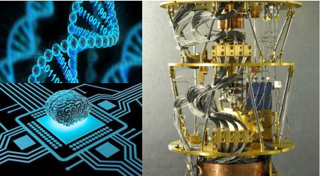
Abstract— This was originally written as an invited “vision” presentation for the eScience 2019 conference, but I decided to present something more focused for that event. Never wanting to let words go to waste I decided to put a revised version here.   It was written as a look back at the period of eScience from 2019 to 2050.   Of course, as it is being published in 2019, it is clearly a work of science fiction, but it is based on technology trends that seem relatively clear. Specifically, I consider the impact of four themes on eScience: the explosion of AI as an eScience enabler, quantum computing as a service in the cloud, DNA data storage in the cloud, and neuromorphic computing.

I.  Introduction

Predictions of the future are often so colored by the present that they miss the boat entirely.   The future, in these visions, tends to look like today but a bit nicer. Looking at images of the future from the 1950s we see pictures of personal helicopters (Figure 1) that clearly missed the mark.   But in some cases, the ideas are not so far off, as in the case of the woman ordering shirts “online” as in Figure 2.

hilicopters5

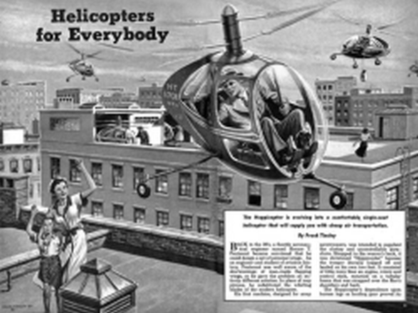
Fig 1. Future personal transportation. Mechanics Illustrated, Jan 1951

videophone2

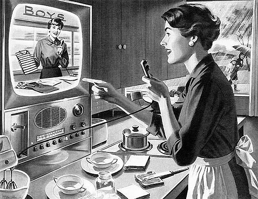
Fig 2. Shopping “online” vision.

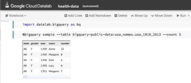
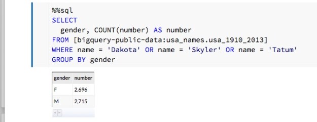
To look at the evolution of eScience in the period from 2019 to 2050, it can help to look at the state of the art in computing in 1960 and ask how much of todays technology can we see emerging there.   My first computer program was written when I was in high school. It was a Fortran version of “hello world” that consited of one line of Fortran per punched card as shown in Figure 3 and the entire program consisted of a deck of 12 cards .

Punched_card2

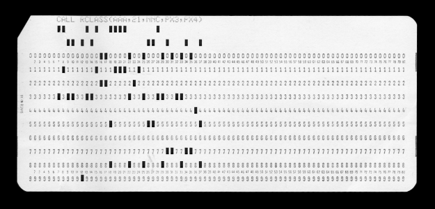
Fig 3.   The Fortran statement CALL RCLASS(AAA,21,NNC, PX3,PX4)

If asked to predict the future then, I might have said that software and data in the years ahead would be stored on a punched paper tape over ten miles long.

Fifty years ago, the high points of computing looked like:

  • The programming language FORTRAN IV was created in 1961.
  • IBM introduced its System/360. A monster machine.
  • Gordon Moore makes an observation about scale in 1965 (that became Moore’s law).
  • IBM created the first floppy disk in 1967.
  • The SABRE database system that was used by IBM to help American Airlines manage its reservations data.
  • In 1970 Edgar Codd came up with Relation Database Idea. It was not implemented until 1974.
  • The Internet: a UCLA student, tries to send “login,” the first message over ARPANET, at 10:30 P.M. on October 29, 1969.  (The system transmitted “l” and then “o” …. and then crashed.)

     What we can extrapolate from this is that mainframe IBM computers will continue to dominate, databases are going to emerge as a powerful tool and there will be a future for computer-to-computer networking, but PCs and web search were not remotely visible on the horizon. The profound implication of Moore’s law would not be evident until the first microprocessors appear in 1979 and the personal computer revolution of the 1980s followed. Those same microprocessors led to the idea that dozens of them could be packaged into a “parallel computer”. This resulted in a period of intense research in universities and startups to build scalable parallel systems. While the first massively parallel computer was the Illiac IV which was deployed at NASA Ames in 1974, it was the work on clusters of microprocessors in the 1980s [1] that led to the supercomputers of 2019. Looking at computing in 1970, few would have guessed this profound transition in computing from mainframes like the System/360 to the massively parallel systems of 2019.

II. eScience from 2019 Forward

A.   The Emergence and Evolution of the Cloud

   The World Wide Web appeared in 1991 and the first search engines appeared in the mid 90s. As these systems evolved, so did the need to store large segments of the web on vast server farms. Ecommerce also drove the need for large data centers. These data centers quickly evolved to offering data storage and virtual machines as a service to external users.   These clouds, as they became known, were designed to serve thousands to millions of concurrent clients in interactive sessions.

   For eScience, clouds provided an important alternative to traditional batch-oriented supercomputers by supporting interactive, data exploration and collaboration at scale. The cloud data centers evolved in several important way. Tools like Google’s Kubernetes was widely deployed to support computation in the form of swarms of microservices built from software containers. Deploying Kubernetes still required allocating resources and configuring systems and microservices are continuously running processes. Serverless computing is a newer cloud capability that avoids the need to configure VMs to support long running processes when they are not needed.

   Serverless computing is defined in terms of stateless functions that respond to events such as signals from remote instruments or changes in the state of a data archive. For examples, an eScience workflow can be automatically triggered when instrument data arrives in the data storage archive. The analysis in the workflow can trigger other serverless function to complete additional tasks.

   The Cloud if 2019 is defined in terms of services and not raw hardware and data storage. These services include

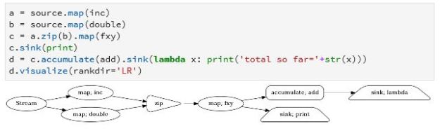
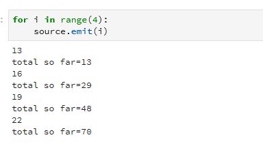
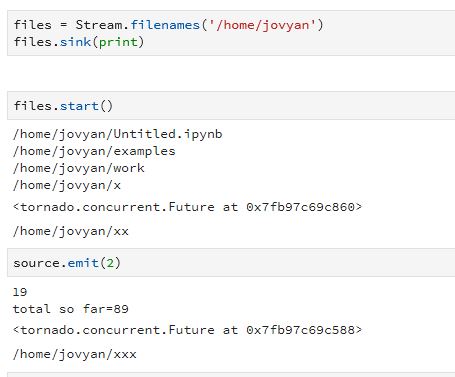
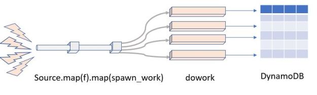
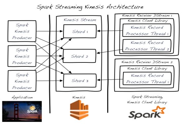
  • Streaming data analytics tools that allow the users to monitor hundreds of live streams from remote instruments.   Edge computing services evolved as a mechanism to off-load some of the analytics to small devices that interposed between the instruments and the cloud.
  • Planet scale databases allow a user to store and search data collections that are automatically replicated across multiple continents with guaranteed consistency.
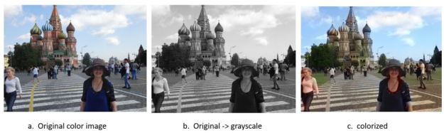
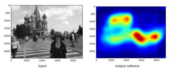
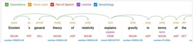
  • Services to support applications of machine learning became widely available across all the commercial public clouds. These services include speech recognition and generation, automatic language translation, computer vision tasks such as image recognition and automatic captioning.

   The architecture of the cloud data centers continued to evolve toward ideas common in modern supercomputers. The first major change was the introduction of software defined networking throughout the data centers. Amazon began introducing GPU accelerators in 2012. This was followed by Google’s introduction of TPU chips to support the computational needs of deep learning algorithms coded in the Tensorflow system. The TPU (figure 4) is a device designed to accelerate matrix multiplication. It is based on systolic computation ideas of the 1980s and has been applied primarily to Google machine learning projects.

Fig 4.   Google TPU v3 architecture. See N. Jouppi, C. Young, N. Patil,  D. Patterson [2, 3].

The most radical evolutionary step has been taken by Microsoft in the Azure cloud. Project Brainwave represents an introduction of a mesh connected layer of FPGA devices that span the entire data center (figure 5).   These devices can be programed to cooperate on parallel execution of lage computational task including serving deep learning models.brainwave-arch
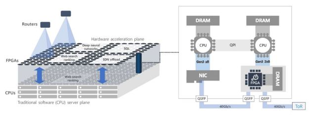
Fig 5. Microsoft FPGA based Project Brainwave [4, 5]

A.   Major Themes Going Forward from 2019

The following pages will describe the four major themes that are going to dominate the ten years forward from 2019.   They are

  • The explosion of AI as an eScience enabler.
  • Quantum computing as a service in the cloud.
  • DNA data storage in the cloud.
  • Neuromorphic computing

 III. AI and eScience

     Machine Learning went through a revolution in the years from 2008 to 2019 due to the intensive work at universities and in companies.   The cloud providers including Google, Microsoft and others were driven by the need improve their search engines. Along the way they had amassed vast stores of text and images. Using this data and the new deep learning technologies they were able to build very powerful language translations systems and image recognition and captioning services that were mentioned above. By 2017, applications to eScience were beginning to emerge.

A.   Generative Neural Networks and Scientific Discovery

     One of the more fascinating developments that arose from the deep learning research was the rise of a special class of neural networks called generative models. The important property of these networks is that if you train them with a sufficiently, large and coherent collection of data samples, the network can be used to generate similar samples. These are most often seen in public as pernicious tools to create fake images and videos of important people saying things they never said.

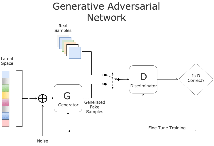
     What these networks are doing is creating a statistical distribution of data that, when sampled, produces data that has properties that match nicely with the input data. When a scientist creates a simulation based on assumed parameters of nature, the simulations is evaluated against the statistical properties of the experimental observations.   Generative models can be used to validate the simulation output in case the data is sparse. One of the most commonly used generative model is the Generative Adversarial Network (GAN) in which to networks are pitted against each other. As shown in Figure 6, a discriminator is trained to recognize the data that is from the real data set and a generator is designed to fool the discriminator. When converged the generator mimics the data distribution of the real data. There are several interesting examples of how generative models have been used in science. We list several in [6], but two that stand out are an application in astronomy and one in drug design.

GAN

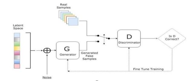
Fig 6. Generative Adversarial Network (GAN) from this site.

    M. Mustafa, and colleagues demonstrate how a slightly-modified standard Generative Adversarial Network (GAN) can be used generate synthetic images of weak lensing convergence maps derived from N-body cosmological simulations [7]. The results illustrate how the generated images match their validation tests, but what is more important, the resulting images also pass a variety of statistical tests ranging from tests of the distribution of intensities to power spectrum analysis.

    However, generative methods do not, by themselves, help with the problem of inferring the posterior distribution of the inputs to scientific simulations conditioned on the observed results, but there is value of in creating ‘life-like’ samples. F. Carminati, G. Khattak, S. Vallecorsa make the argument that designing and testing the next generation of sensors requires test data that is too expensive to compute with simulation . A well-tuned GAN can generate the test cases that fit the right statistical model at the rate needed for deployment [8].

     In the area of drug design, Shahar Harel and Kira Radinsky have used a generative model to suggest chemical compounds that may be used as candidates for study [9]. They start with a prototype compound known to have some desirable properties. This is expressed as sequence and fed to a layer of a convolutional network that allow local structures to emerge as  shorter vectors that are concatenated. A final all-to-all layer is used to generate sequence of mean and variance vectors for the prototype. his is fed to a “diversity layer” which add randomness as shown in Figure 7.

drug-network

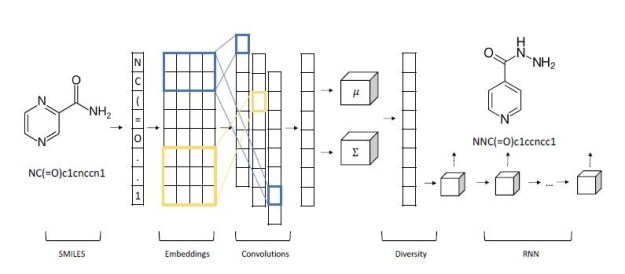
Fig 7. Shahar Harel and Kira Radinsky multi-layer generative netowork for drug design.

       The decoder is an LSTM-based recurrent network which generates the new molecule. The results they report are impressive. In a one series of experiments they took as prototypes compounds from drugs that were discovered years ago, and they were able to generate more modern variations that are known to be more powerful and effective. No known drugs were used in the training.

B.   Probabilistic Programming and Bayesian Inference

     For very large experiments such as those conducted in the Large Hadron Collider, the scientists are interested in testing their models of the universe based the record of particle collisions that were generated.   It is often the case that the scientists have a detailed simulation of the experimental system based on the current theoretical models of physics that are involved. These models are driven by setting parameters that correspond to assumptions about nature. When they run the experiment, they see new behaviors in the data, such as new particles emerging from collisions, and they would like to see which parameters when fed to the simulation can produce the output that corresponds to the experimental results. In other words, the simulation is a function taking parameters x to outputs y and the interesting question is given the outputs what the corresponding values for x. This is an inverse problem that is notoriously difficult to solve for large scientific problems. In terms of Bayesian statistics, they are interested in the posterior distribution P(x | y) where y is the experimental statistics.

     In 2018 and later researchers began to study programming languages designed to express and solve problems like these. Pyro [10], Tensorflow Probability [11], and the Julia-based Gen [12] are a few of the Probabilistic Programing Languages (PPLs) introduced in 2019. One of the ideas in these languages is to build statistical models of behavior where program variables represent probability distributions and then, by looking at traces of the random choices associated with these variables during execution, one can make inferences about the random behaviors that influence outcomes.

     These languages have been put in use in industries such as finance, their role in eScience is now becoming apparent.    A. Güneş Baydin, et al. showed that PPLs can be used in very large Bayesian analysis of data from an LHC use case. Their approach allows a PPL too couple directly to existing scientific simulators through a cross-platform probabilistic execution protocol [13].

     Probabilistic programming with PPLs will go on to become a standard tool used by eScientists.

C.   AI-based Research Assistant

      2018 was the year of the smart on-line bot and smart speaker. These were cloud based services that used natural language interfaces for both input and output. The smart speakers, equipped with microphones listen for trigger phrases like “Hello Siri” or “hello Google” or “Alexa” and recorded a query in English, extracted the intent and replied within a second. They could deliver weather reports, do web searches, keep your shopping list and keep track of your online shopping.

     The impact of this bot technology will hit eScience when the AI software improves to the point that every scientist, graduate student and corporate executive had a person cloud-based research assistant. Raj Reddy calls these Cognition Amplifiers and Guardian Angels. Resembling a smart speaker or desktop/phone app, the research assistant is responsible for the following tasks:

  • Cataloging research data, papers and articles associated with its owner’s projects. The assistant will monitor the research literature looking for papers exploring the same concepts seen in the owner’s work.
  • Coordinate meetings among collaborators and establish coordination among other research assistants.
  • Automatically sifting through other data from collaborators and open source archives that may be of potential use in current projects.
  • Understanding the mathematical analysis in the notes generated by the scientist and using that understanding to check proofs and automatically propose simulators and experiment designs capable of testing hypotheses implied by the research.

     From the perspective of 2019 eScience, the claim that the Research Assistant of the future will be able to derive simulations and plan experiments may seem a bit “over the top”. However, progress on automatic code completion and generation was making great strides in 2019. Transformers [16] provide a second generation of sequence-to-sequence AI tools that outpaced the recurrent neural networks previously used.   Advances in programming tools based on similar technology show that AI can be used to generate code completions for C# method calls based on deep semantic mining of online archives of use cases.

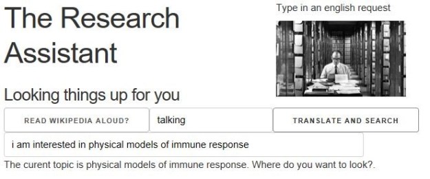
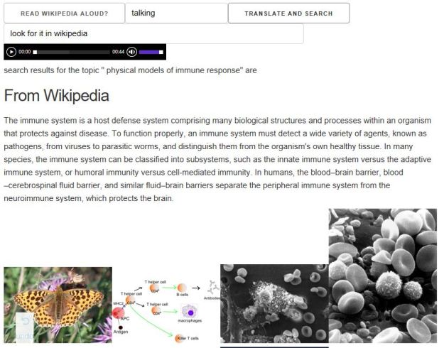
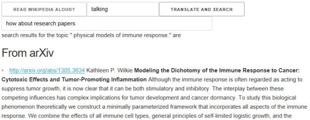
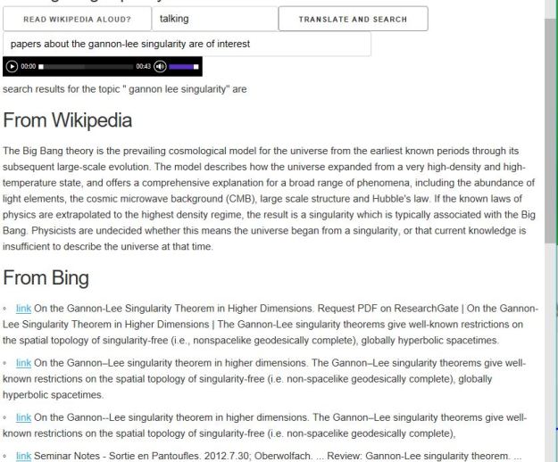
     We built a toy demo of the Research Assistant in [14] that could take natural language (spoken or typed) input and find related research articles from Bing, Wikipedia and ArXiv (see Figure 6.)

res-asst4

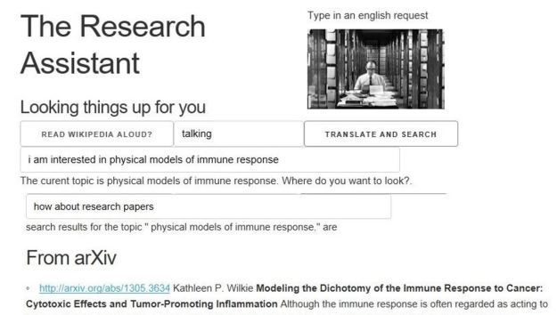
    Fig 6. Demo cloud-based “research assistant” [14]

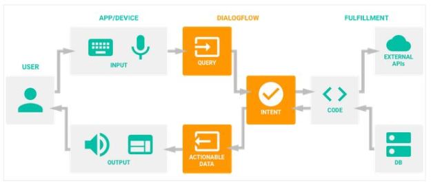
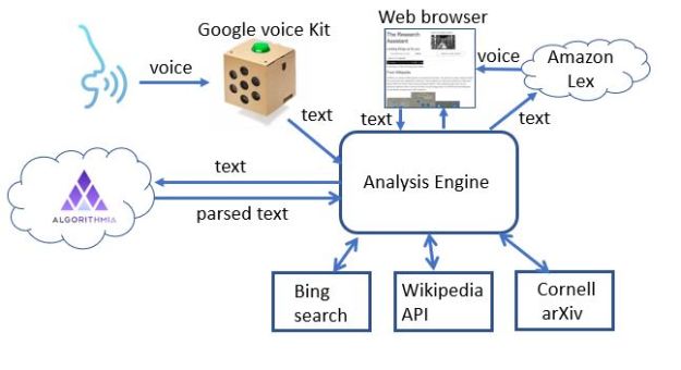
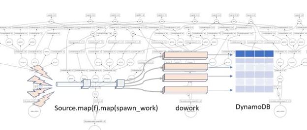
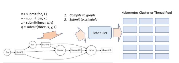
     This demo prototype research assistant was built by composing a few cloud tools as shown in Figure 7. A much more sophisticated version can be built using a modern chatbot tool like RASA, but that will not address everything that is needed to reach the final goal.

Ra-components

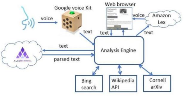
Fig 7. The toy research assistant demo is hosted an “elegant” cardboard container from Google’s voice kit running a python script on raspberry Pi. It invokes Googles speech to text, a text analysis service running on Algorithmia and uses Amazon’s Lex to generate voice. Depending on context, calls are made to Bing, Wikipedia or ArXiv.

     While this demo was a toy, there has been serious work over the last few years to make progress on this topic. In 2018, Google introduced its Dataset Search service to provide easy data set discovery. The work of the Allen Institute for AI stands out [15]. Their Semantic Sanity project is a sophisticated research search engine that allows you to tell it basic topics that interest you and it will monitor ArXiv looking for important related contributions.   Aristo is “an intelligent system that reads, learns, and reasons about science”. It can reason about diagrams, math and understand and answer elementary school science questions.

     One important problem that must be solved is extracting non-trivial mathematical concepts from research papers and notes so that similar papers can be found. In addition to Semantic Sanity, there is some other early related work on this problem. For example, researchers are using unsupervised neural net to sift through PubChem and uses NLP techniques to identify potential components for materials synthesis [22].

 IV. The Rise of Quantum in the Cloud

     Long viewed as a subject of purely theoretical interest, quantum computing emerged in 2018 as a service in the cloud. By 2019, Rigetti, IBM, D-Wave and Alibaba had live quantum computing services available.   Google and Microsoft followed soon after that.   The approaches taken to building a quantum computer differed in many respects.

     The basic unit of quantum computing is the qubit which obeys some important and non-intuitive laws of physics. Multiple qubits can be put into an “entangled” state in which an observation about one can effect the state of the others even when they are physically separated.   One can apply various operators to qubits and pairs of qubits to form “logical” circuits and these circuits are the stuff of quantum algorithms. A fact of life about quantum states is that once you measure them, they are reduced to ordinary bits. However, the probability that a bit is reduced to a zero or a one is determined by the unmeasured quantum state of the system. A good quantum algorithm is one in which the quantum circuit produces outputs with a probability distribution that makes solving a specific problem very fast.

     The first important quantum computations involved solving problems in quantum chemistry. In fact, this was the role that Richard Feynman had suggested for a quantum computer when he first came up with the idea in the 1980s. The other area of eScience that quantum computers excelled at was certain classes of optimization problems.

     Early quantum computers are program by literally composing the quantum gates as illustrated in Figure 8.quantum-circuit

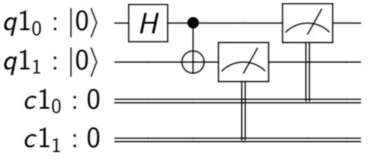
Fig 8. A simple quantum circuit to create an entangled pair of two qubits and measure the result

     Programming tools to build such circuits include IBM’s IBM-Q qiskit and Microsoft’s Q# language and compiler. The IBM hardware was based what they call “noisy intermediate-scale quantum computers (NISQ)”. As shown in Figure 9, the induvial qubits are non-linear oscillators. Tuned superconducting resonator channels are used for readout. Also, the qubits are tied together by additional superconducting channelsibm-qubits

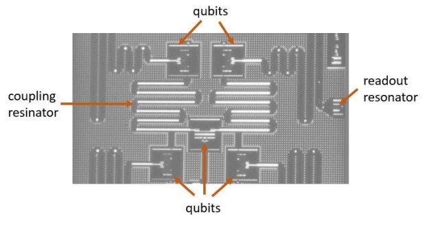
Fig 9 An early 5-qubit IBM-Q computational unit. Source: IBM-Q website.

     One problem with early quantum systems is that the qubits are very susceptible to noise and degrade quickly.   In other words, the error rate of quantum algorithms can be very high. The deeper the quantum circuit (the number of layers of “gates”), the more noise. A way around this is to add error-correcting redundancy into the circuit, but this means more qubits are required.   Quantum volume refers to a measure of the number of qubits needed for the error-corrected circuit times the depth of the corrected circuit. Unfortunately, early quantum computers had very low bounds on achievable quantum volume.

Microsoft took a different approach to building qubits that are based on the topological property of woven threads. These are much more noise resistant and hence capable of building deeper circuits with less error correction.

IV.  DNA-Based Storage

     There are two problems with 2019 era storage technologies.   First, it was not very stable. Data degrades and storage devices fail. Second, there was not enough storage capacity to capture the data that was being generated.   2.5 quintillion bytes of data was generated each day in 2018. Even if you cast out 99.9% of this as being of no long-term value, the remainder still leaves 2.5e+15 bytes per day. The amount of data stored in the cloud in 2018 was 1.0e+18 (an exabyte). In other words, the cloud only held 400 days’ worth of the important data. Obviously, another order or magnitude or more of the data needed to be discarded to allow the data centers time to expand to contain this growth. A new storage technology was needed.

     DNA storage was first proposed in the 1960, but not much happened with the idea until 1988 when researchers from Harvard stored an image in the DNA of e.coli. By 2015 researchers at Columbia University published a method that allowed the storage of 215 petabytes (2.15e+17) of data per gram of DNA. And DNA is very stable over long periods of time. While this was promising, there was still a big problem.   The encoding and decoding of the data were still an expensive manual process and it was not practical to have lab scientists running around in the back rooms of data centers managing wet processes.

        In 2019, researchers at the University of Washington and Microsoft demonstrated an automated lab that could encode and decode data to DNA without human hands. The system works by converting the ones and zeros of digital data into the As, Ts, Cs and Gs that make up the building blocks of DNA. These encoded sequences are then fed into synthesizing systems. Their next breakthrough was to reduce the entire “lab” to a chip that uses microfluidics to route droplets of water around a grid to enact the needed chemistry steps. They also produced a sophisticated software stack called puddle that allow the scientist to program this with conventional high-level languages [20].

      Other research has demonstrated ways in which DNA encoded data could be searched and structured in ways like relational databases.   As the costs came down, this became the standard cloud storage technology.

VI. Neuromorphic Computing

     It was long a dream of computer designers to build systems that mimicked the connectome of the biological brain. A major research initiative in Europe, the Human Brain Project, looked at the possibility of simulation a brain on traditional supercomputers. As that proved unrealistic, they turned to the study of special hardware devices that can simulate the behavior of neuron. Technology to build artificial neurons progressed in university and industry labs. The Stanford neurogrid can simulate six billion synapses.   In 2017 Intel introduced the Loihi neuromorphic research test chip. The device is a many-core mesh of 128 neuromorphic cores and each of which contains 1,024 primitive spiking neural units. The neural units are current-based synapse leaky integrate-and-fire neurons [21].

     In addition to the Loihi chip, Intel has released Pohoiki Beach, a system comprised of 64 Loihi chips and a substantial software stack to allow application development. Because overall power consumption is 100 times lower than GPU based neural networks, Intel’s application target is autonomous vehicles and robots. While full realization of true biological brain-like functionality may not be realized until the 2nd half of the 21st century, it is none the less an exciting step forward.

 VII.   Conclusions

     EScientists in 2019 found themselves at an important inflection point in terms of the technology they could deploy in doing science.   The cloud has evolved into a massive on-line, on-demand, heterogeneous supercomputer. It not only supports traditional digital simulation; it will also support hybrid quantum-digital computation.   It will soon allow applications to interact with robotic sensor nets controlled by neuromorphic fabrics. Storage of research data will be limitless and backed up by DNA based archives.

     One of the most remarkable features of computing in the 21st century has been the evolution of software. Programming tools have evolved into very deep stacks that have used and exploited AI methods to enable scientific programmer to accomplish more with a few lines of Julia in a Juypter notebook than was remotely possible programming computers of 1980. New probabilistic programming languages that combine large scale simulation with deep neural networks show promise of making Bayesian inference an easy to use used tool in eScience.

     The role of AI was not limited to the programming and execution of eScience experiments. Users of the AI research assistants in 2050 can look back at the “smart speakers” of 2019 and view them as laughably primitive as the users of the 2019 World Wide Web looked back at the 1970s era where computers were driven by programs written on decks of punched cards.

References

  1. G. Fox, R. Williams, P. Massina, “Parallel Computing Works!”, Morgan Kauffman, 1994.
  2. N. Jouppi, C. Young, N. Patil, D. Patterson, “A Domain-Specific Architecture for Deep Neural Networks”, Communications of the ACM, September 2018, Vol. 61 No. 9, Pages 50-59
  3. https://cloud.google.com/tpu/docs/images/tpu-sys-arch3.png
  4. Chung, et al. “Serving DNNs in Real Time at Datacenter Scale with Project Brainwave.” IEEE Micro 38 (2018): 8-20.
  5. Fowers et al., “A Configurable Cloud-Scale DNN Processor for Real-Time AI,” 2018 ACM/IEEE 45th Annual International Symposium on Computer Architecture (ISCA), Los Angeles, CA, 2018, pp. 1-14
  6. D. Gannon, “Science Applications of Generative Neural Networks”, https://esciencegroup.com/2018/10/11/science-applications-of-generative-neural-networks/, 2018
  7. Mustafa, et. al. “Creating Virtual Universes Using Generative Adversarial Networks” (arXiv:1706.02390v2 [astro-ph.IM] 17 Aug 2018)
  8. Carminati, G. Khattak, S. Vallecorsa, “3D convolutional GAN for fast Simulation”, https://www.ixpug.org/images/docs/IXPUG_Annual_ Spring_Conference_2018/11-VALLECORSA-Machine-learning.pdf
  9. Harel and K. Radinsky, “Prototype-Based Compound Discovery using Deep Generative Models” http://kiraradinsky.com/files/acs-accelerating-prototype.pdf
  10. Bingham, et al, “Pyro: Deep universal probabilistic programming.” Journal of Machine Learning Research (2018).
  11. Tensorflow Probability, https://medium.com/tensorflow/an-introduction-to-probabilistic-programming-now-available-in-tensorflow-probability-6dcc003ca29e
  12. Gen, https://www.infoq.com/news/2019/07/mit-gen-probabilistic-programs
  13. Güneş Baydin, et al, “Etalumis: Bringing Probabilistic Programming to Scientific Simulators at Scale”, arXiv:1907.03382v1
  14. Gannon, “Building a ‘ChatBot’ for Scientific Research”, https://esciencegroup.com/2018/08/09/building-a-chatbot-for-scientific-research
  15. Allen Institute for AI, Semantic Sanity and Aristo, https://allenai.org/demos
  16. Vaswani et al., “Attention Is All You Need”, arXiv:1706.03762v5
  17. Chong, Hybrid Quantum-Classical Computing https://www.sigarch.org/hybrid-quantum-classical-computing/
  18. Shaydulin, et al., “A Hybrid Approach for Solving Optimization Problems on Small Quantum Computers,” in Computer, vol. 52, no. 6, pp. 18-26, June 2019.
  19. Takahashi, B. Nguyen, K. Strauss, L. Ceze, “Demonstration of End-to-End Automation of DNA Data Storage”, Nature Scientific Reports, vol. 9, no. 1, pp. 2045-2322, 2019
  20. Wellsey, et al., “Puddle: A Dynamic, Error-Correcting, Full-Stack Microfluidics Platform”, ASPLOS’19 , April 13–17, 2019.
  21. Intel Loihi Neurmorphic Chip. https://en.wikichip.org/wiki/intel/loihi
  22. E. Kim, et al., “Materials Synthesis Insights from Scientific Literature via Text Extraction and Machine Learning”, Chem. Mater. 2017 29219436-944

Building a “ChatBot” for Scientific Research

We can use Alexa, Cortana and Siri to check the weather, stream our favorite music and lookup facts like “who directed Casablanca?” But if I want to find all the research on quantum entanglement in the design of topological quantum computers, these services will fall short.   If, in addition, I want these articles cataloged in my personal archive and the citations automatically pulled I need a much more robust digital assistant.  Raj Reddy talks about a broader and more pervasive future for digital assistant he calls Cognition Amplifiers and Guardian Angels.  In this post we look at chatbots and their limitations and show how to build a simple, voice-driven scientific metasearch tool we call the research assistant.  Finally, we discuss the next phase of research assistant.

Smart Speakers and Chatbots.

The revolution in “smart speaker” digital assistants like Siri, Amazon Echo, Google Home is showing us the power of voice to provide input to smart cloud services.   These assistants can take notes, tell us the weather conditions, place on-line orders for us and much more.   I even allow Microsoft’s Cortana to read my email.  If I send the message “I’ll get back to you tomorrow” to a friend, Cortana will remind me the next day that a response is needed.  Amazon allows people to add “skill” (additional capabilities) to there Alexa system.  These smart speakers are designed around open-ended question-response scenario.  These assistants leverage very powerful speech-to-text technology and semantic analysis systems to extract a query or command.  The query answers are derived from web-data analysis and the commands are to a limited number of native services (or external skills).

A chatbot is a system that engages the user in a dialog.   They go beyond the question answering smart speakers and are usually designed to help people interact with the services of a specific company or agency.   The Google, IBM, Amazon and Microsoft have all introduced cloud services to help anybody build a chatbot.   These services guide you through the process of building and training a chatbot.   A good example is Google’s Dialogflow.   Using this tool to create a bot, you specify three things:

  • Intents – which are mapping between what the user says and how you wish the system to respond.
  • Entities – that are the categories of subjects that your bot understands. For example, if you bot is a front end to your clothing store, one category of entity my be product type: shoes, dress, pants, hats,  and another entity might be size: large, xl, small, medium,  and another might be color.
  • Context – This is knowledge obtained by the bot during the course of the conversation. For example, the name of the user, or the users favorite shoe color.

The goal of the bot is to extract enough information from the user to take a meaning action such as fulfilling an order.   The hard part is designing the intents so that a dialog can lead to the desired conclusion.  The resulting sysgtem is called an agent and the flow of action is illustrated in Figure 1.  It might start with ‘Good morning, how can I help you?’   and end with a summary of the discussion.  As the programmer you need to supply as many possible variations on possible user questions and responses as possible.  And you must annotate these with makers where your entities can be extracted.    Your examples are used in a training phase that maps your intents and entities together and builds a model that will learn variations on the input and not repeat the same sequence of responses each time, so it seems less robotic to the user.

Amazon’s Lex provides a similar service that also integrates with their lambda services.  Microsoft has the Azure Bot Service and IBM has Watson assistant chatbot tools.

dialogflow

Figure 1. Google Dialogflow Agent architecture.

These tools are all designed to help you build a very focused conversation with the user about a very narrow universe such as the on-line part of a business.   But this raises the question, can one build a chat bot that can carry out an open-ended conversation.  Perhaps one that could pass the Turing test?   The research literature on the subject is growing and deep learning tools like recurrent and convolutional neural networks have been applied to the problem (see https://arxiv.org/pdf/1606.07056.pdf , https://arxiv.org/pdf/1605.05110.pdf and more).   Unfortunately chatbots designed to engage in open-ended conversation have only had a limited success.   Xiaoice is one that interacts with users on the Chinese micro blogging service Weibo.  The problem is that while it sounds like conversation, it is mindless.  Microsoft’s Tay was an English language version that operated on Twitter until it was taken down after only 16 hours because of the unfortunate language it had learned.  A successor Zo seems to be working better, but it does not produce conversations with intellectual content.

There is an excellent pair of articles by Denny Britz about the role of deep learning for conversational assistants.   He make the point that for open-ended conversations (he calls them open-domain) the challenges are large compared to the fixed domain chatbots because so much more world knowledge is required.

Cognition Amplifiers and the Research Assistant.

In the spring of 2018 Raj Reddy gave the keynote presentation at the IEEE services congress.  His topic was one he has addressed before and it clearly resonated with the audience.   He described Cognition Amplifiers and Guardian Angels.  He defined a Cognition Amplifier (COG) as a Personal Enduring Autonomic Intelligent Agent that anticipates what you want to do and help you to do it with less effort. A Guardian Angel (GAT) is a Personal Enduring Autonomic Intelligent Agent that discovers and warns you about unanticipated events that could impact your safety, security and happiness.

Consider now the application of the Cognition Amplifier to scientific research.   If you are working on writing a research paper, you may wish your autonomic research assistant to provide a fast and accurate search of the scientific literature for a specific list of scientific concepts. In fact, as you write the paper, the assistant should be able to pick up the key concepts or issues and provide a real-time bibliography of related papers and these should be stored  and indexed in a private space on the cloud.  Extracting key phrases from technical documents is already a heavily research field so applying this technology to this problem is not a great leap.   However, key phrase extraction is not the whole challenge.   Take sentence “It seems that these days investors put a higher value on growth than they do on profitability”.  The categorical topic is value of growth vs profitability – investor opinions which is not simply a key phrase, but a concept and we need the research assistant to look for concepts.    Your research assistant should always understand and track the context of your projects.

Finally, a good research assistant for science should be able to help with the analytical part of science.  For example, it should help locate public data in the cloud related to experiments involving your topics of interest.   The assistant should be able to help formulate, launch and monitor data analysis workflows. Then coordinate and catalog the results.

And, of course, if your autonomous research assistant is also a Guardian Angel, it will also keep you informed of grant reporting deadlines and perhaps pull together a draft quarterly report for your funding agency.

I fully expect that it is possible to build such an agent in the years ahead.   However, the remainder of this article is a simple demo that is a far cry from the full research assistant agent described above.

The Research Assistant Metasearch Tool.

In the following paragraphs we describe a very simple voice-driven agent that can be used to look for research articles about scientific topics.  We also show how such a system can be assembled from various simple devices and cloud services.   The system we describe is not very sophisticated.  In fact it is not much better than Cortana at finding things given English input sentence.  However we feel it does illustrate the architecture of a voice-driven agent that can be built by gluing together easy to use cloud services.

Our scenario is a researcher sitting near the device and asking about very specific research topics such as “physical models of immune response” or “programming a topological quantum computer”.    We assume the user wants a spoken response if that response is simple, but we also realize that this is impractical if the system is creating a list research journal papers.  To address this issue, the system also has a display in a web browser.  (We note that the Cortana and Google assistant do the same if the response is a list.)

Figure 2 illustrates the basic architecture of the system.

architectureofRA

Figure 2.  The architecture of the research assistant.

The components of the system are:

  1. The voice-to-text translator. Here we use a simple voice kit from google.   This consists of some special hardware and a raspberry pi 2 computer all packaged in an elegant cardboard box.  You wake the system up by pressing the botton on top and speak.   The audio is captured and sent to the google voice service for transcription and it is returned as a text string.
  2. The next step is to parse the text string into the components that will allow us to extract the topics of the query.  This is another cloud service call.  This time it is to Algorithmia.com and the service is called key phrases.  (we wrote about this in a previous article.)  The service takes English sentences and invoked Googles ParsyMcParseface (another Algorithmia.com AI service) and returns a list composed of three types of phrases: subject (s), actions (a) and objects (o).  It also flags prepositional phrases with a “/” character.   So for example, “I am interested in physical models of immune response” returns

          [‘s: I ‘, ‘a: am ‘,  ‘o: interested /in physical models /of immune response.’]

  1. The analysis engine is a 500-line Python Dash-based web server that extracts the topics and a few other items of interest and decides how to search and display the results on the browser. There are three web services used for the search: Wikipedia,  Bing and Cornell’s ArXiv service[1].  To see how this works, consider the example the sentence “research papers by Michael Eichmair about the gannon-lee singularity are of interest“. The analysis engine detects the topic as the gannon-lee singularity and Michael Eichmar as the author.  The fact that research papers are of interest indicates that the we should look in the Cornell ArXiv repository of papers.   (The results for this query are at the end of this section).    (Truth in advertising: our parser and analysis are far from perfect.   For example, “tell me about Deep Learning”   vs “tell me about deep learning” yield two different parses.  The first yields

            [‘a: tell ‘, ‘o: me /about Deep Learning ‘]

           which is fine. But the second gives us

          [‘a: tell ‘, ‘o: me about deep ‘, ‘a: learning ‘]

           which causes the analysis to fail. )

  1. Finally, we use the Amazon Lex services to generate the audio reading of the Wikipedia results. If you have an aws account, the Python API is easy to use.

Examples

Figure 3 illustrates the interface.  We have started with the statement “I am interested in physical models of immune response.”

fig3-chatbot

Figure 3.   The interface provides a switch to allow the Wikipedia response to read aloud.   In this case we have typed the English statement of intent into the query box and hit the “Translate and Search” button.

We respond with the phrase “look for it in Wikipedia” and get the result in figure 4.    Following that response, we say “how about research papers” and we get the response in figure 5.

webpage3

Figure 4.   The response to “look for it in wikipedia”.  A short summary from Wikipedia is extracted along with related images found on the subject.  The spoken response is controlled by the audio control  at the top of the response.

webpage4

Figure5.   The mention of research papers suggest that we should consult the Cornell library arXiv.    Shown above is only the first result of 10 listed on the page.

Returning to the example mentioned above “research papers by Michael Eichmair about the gannon-lee singularity are of interest” we get the following results.   You will notice that the Wikipedia result is a default hit for “big bang singularity” and not directly related to the precise query.  The Bing results and the ArXiv hits are accurate.

webpage5

Figure 6.  Results for the query “research papers by Michael Eichmair about the gannon-lee singularity are of interest”.  (This page was slightly edited to shorten the list of Bing results.)

The system has a limited capability to pull together concepts that are distributed over multiple sentences.  For example the input string “what are anyons?   How do they relate to topological quantum computation?” will build the topic “anyons topological quantum computation”.

If you are interested in trying to use the system point your browser here.  I will try keep it up and running for a few months. There is no voice input because that requires a dedicated Google voice kit on your desk.   You need to decide if you want to have a playback of the audio for Wikipedia summaries.   If you don’t want it, simply press the “Read Aloud” button.  Then enter a query and press the “Translate and Search” button.   Here are some samples to try:

  1. what did they say about laughter in the 19th century?
  2. are there research papers about laughter by Sucheta Ghosh?
  3. what can you tell me about Quantum Entanglement research at Stanford? (this one fails!)
  4. what can you tell me about research on Quantum Entanglement at Stanford?
  5. what are anyons? How do they relate to topological quantum computation?
  6. Who was Winslow Homer? (this one give lots of images)
  7. I am interested in gravitational collapse. (respond with web, Wikipedia or arxiv)

As you experiment, you will find MANY errors.  This toy is easily confused.   Please email me examples that break it.  Of course, feedback and suggestions are always welcome.  I can make some of the source code available if there is interest. However, this is still too unreliable for public github.

[1] There are other arguably superior sources we would like to have used.  For example, Google Scholar would be perfect, but they have legal restrictions on invoking that service from an application like ours.  Dblp is also of interest but it is restricted to computer science.

Parallel Programming in the Cloud with Python Dask

I am always looking for better ways to write parallel programs.  In chapter 7 of our book “Cloud Computing for Science and Engineering” we looked at various scalable parallel programming models that are used in the cloud.   We broke these down into five models: (1) HPC-style “Single Program Multiple Data” (SPMD) in which a single program communicates data with copies of itself running in parallel across a cluster of machines, (2) many task parallelism that uses many nearly identical workers processing independent data sets, (3) map-reduce and bulk synchronous parallelism in which computation is applied in parallel to parts of a data set and intermediate results of a final solution are shared at well defined, synchronization points,  (4) graph dataflow transforms a task workflow graph into sets of parallel operators communicating according to the workflow data dependencies and (5) agents and microservices  in which a set of small stateless services process incoming data messages and generate messages for other microservices to consume.  While some applications that run in the cloud are very similar to the batch style of HPC workloads, parallel computing in the cloud is often driven by different classes application requirements.  More specifically, many cloud applications require massive parallelism to respond external events in real time.  This includes thousands of users that are using apps that are back-ended by cloud compute and data.   It also includes applications that are analyzing streams of data from remote sensors and other instruments.   Rather than running in batch-mode with a start and end, these applications tend to run continuously.

A second class of workload is interactive data analysis.   In these cases, a user is exploring a large collection of cloud resident data.   The parallelism is required because the size of the data: it is too big to download and if you could the analysis would be too slow for interactive use.

We have powerful programming tools that can be used for each of the parallel computing models described above but we don’t have a single programming tool that support them all.   In our book we have used Python to illustrate many of the features and services available in the commercial clouds.  We have taken this approach because Python and Jupyter are so widely used in the science and data analytics community.  In 2014 the folks at Continuum (now just called Anaconda, Inc) and a several others released a Python tool called Dask which supports a form of parallelism similar to at least three of the five models described above.  The design objective for Dask is really to support parallel data analytics and exploration on data that was too big to keep in memory.   Dask was not on our radar when we wrote the drafts for our book,  but it certainly worth discussing now.

Dask in Action

This is not intended as a full Dask tutorial.   The best tutorial material is the on-line YouTube videos of talks by Mathew Rocklin from Anaconda.   The official  tutorials from Anaconda are also available.  In the examples we will discuss here we used three different Dask deployments.  The most trivial (and the most reliable) deployment was a laptop installation.  This worked on a Windows 10 PC and a Mac without problem.  As Dask is installed with the most recent release of Anaconda, simply update your Anaconda deployment and bring up a Jupyter notebook and “import dask”.    We also used the same deployment on a massive Ubuntu linux VM on a 48 core server on AWS.  Finally, we deployed Dask on Kubernetes clusters on Azure and AWS.

Our goal here is to illustrate how we can use Dask to illustrate several of the cloud programming models described above.    We begin with many task parallelism, then explore bulk synchronous and a version of graph parallelism and finally computing on streams.  We say a few words about SPMD computing at the end, but the role Dask plays there is very limited.

Many Task Parallelism and Distributed Parallel Data Structures

Data parallel computing is an old important concept in parallel computing.  It describes a programming style where a single operation is applied to collections of data as a single parallel step. A number of important computer architectures supported data parallelism by providing machine instructions that can be applied to entire vectors or arrays of data in parallel.  Called Single instruction, multiple data (SIMD) computers, these machines were the first supercomputers and included the Illiac IV and the early Cray vector machines.  And the idea lives on as the core functionality of modern GPUs.   In the case of clusters computers without a single instruction stream we traditionally get data parallelism by distributed data structures over the memories of each node in the cluster and then coordinating the application of the operation in a thread on each node in parallel.   This is an old idea and it is central to Hadoop, Spark and many other parallel data analysis tools.   Python already has a good numerical array library called numpy, but it only supports sequential operations for array in the memory of a single node.

Dask Concepts

Dask computations are carried out in two phases.   In the first phase the computation is rendered into a graph where the nodes are actual computations and the arcs represent data movements.   In the second phase the graph is scheduled to run on a set of resources.  This is illustrated below.  We will return to the details in this picture later.

dask-workflow

Figure 1.  Basic Dask operations: compile graph and then schedule on cluster

There are three different sets of “resources” that can be used.   One is a set of threads on the host machine.   Another is a set of process and the third is a cluster of machines.   In the case of threads and local processes the scheduling is done by the “Single machine scheduler”.   In the case of a cluster it called the distributed cluster.  Each scheduler consumes a task graph and executes it on the corresponding host or cluster.   In our experiments we used a 48 core VM on AWS for the single machine scheduler. In the cluster case the preferred host is a set of containers managed by Kubernetes.   We deployed two Kubernetes clusters:  a three node cluster on Azure and a 6 node cluster on AWS.

Dask Arrays, Frames and Bags

Python programmers are used to numpy arrays, so Dask takes the approach to distributing arrays by maintaining as much of the semantics of numpy as possible.  To illustrate this idea consider the following numpy computation that creates a random 4 by 4 array, then zeros out all elements lest than 0.5 and computes the sum of the array with it’s transpose.

x = np.random.random((4,4))
x[x<0.5] = 0
y = x+x.T

We can use Dask to make a distributed version of the same matrix and perform the same computations in parallel.

Import dask.array as da
x = da.random.random(size = (4,4), chunks =(4,1))
x[x<0.5] = 0
y = x+x.T

The important new detail here is that we give explicit instructions on how we want the array to be distributed by specifying the shape of the chunks on each node.   In this case we have said we want each “chunk” to be a 4×1 slice of the 4×4 array.   We could have partitioned it into square blocks of size 2×2.   Dask takes care of managing each chunk and the needed communication between the processes that handle each chunk.   The individual chunks are managed on each thread/process/worker as numpy arrays.

As stated above, there are two parts to a dask computation.   The first phase is the construction of a graph representing the computation involving each chunk. We can actually take a look at the graph.   For example, in the computation above we can use the “visualize()” method as follows.

y = x+x.T
y.visualize()

big-transpose

Figure 2.   Sample Dask Graph for x+x.T

The nodes represent data or operations and the lines are data movements from one node to another.  As can be seen this is a rather communication intensive graph.   This is becase the transpose operation requires element on the rows (which are distributed) must be moved to columns on the appropriate node to do the addition.  The way we chunck the array can have a huge impact on the complexity of the distributed computation.  For example, 2×2 chuncking makes this one very easy.   There are 4 chunks and doing the transpose involves only a simple swap of the “off diagonal” chunks.   In this case the graph is much simpler (and easier to read!)

small-transpose

Figure 3.  Task graph for x+x.T with 2×2 chunking of data

The second step for Dask is to send the graph to the scheduler to schedule the subtasks and execute them on the available resources. That step is accomplished with a call to the compute method.

y.compute()

Dask arrays support almost all the standard numpy array operations except those that involve complex communications such as sorting.

In addition to numpy-style arrays, Dask also has a feature called Dask dataframes that are distributed versions of Pandas dataframes.   In this case each Dask dataframe is partitioned by blocks of rows where each block is an actual Pandas dataframe.  In other words, Dask dataframes operators are wrappers around the corresponding Pandas wrappers in the same way that Dask array operators are wrappers around the corresponding numpy array operators.    The parallel work is done primarily by the local Pandas and Numpy operators working simultaneously on the local blocks and this is followed by the necessary data movement and computation required to knit the partial results together.  For example, suppose we have a dataframe, df, where each row is a record consisting of a name and a value and we would like to compute the sum of the values associated with each name.   We assume that names are repeated so we need to group all records with the same name and then apply a sum operator.  We set this up on a system with three workers.  To see this computational graph we write the following.

df.groupby(['names']).sum().visualize()

groupby

Figure 4.  Dataframe groupby reduction

As stated earlier, one of the motivations of Dask is the ability to work with data collections that are far too large to load on to your local machine.   For example, consider the problem of loading the New York City taxi data for an entire year.    It won’t fit on my laptop.   The data for is for 245 million passenger rides and contains a wealth of information about each ride.  Though we can’t load this into our laptop we can ask dask to load it from a remote repository into our cloud and automatically partition it using the read_csv function on the distrusted dataframe object as shown below.

taxi1

Figure 5.  Processing Yellow Cab data for New York City

The persist method moves the dataframe into memory as a persistent object that can be reused without being recomputed.  (Note:  the read_cvs method did not work on our kubernetes clusters because of a missing module s3fs in the dask container, but it did work on our massive shared memory VM which has 200 GB of memory.)

Having loaded the data we can now follow the dask demo example and compute the best hour to be a taxi driver based on the fraction of tip received for the ride.

taxi3

Figure 6.  New York City cab data analysis.
As you can see, it is best to be a taxi driver about 4 in the morning.

A more general distributed data structure is the Dask Bag that can hold items of less structured type than array and dataframes.   A nice example http://dask.pydata.org/en/latest/examples/bag-word-count-hdfs.html illustrates using Dask bags to explore the Enron public email archive.

Dask Futures and Delayed

One of the more interesting Dask operators is one that implements a version of the old programming language concept of a future   A related concept is that of lazy evaluation and this is implemented with the dask.delayed function.   If you invoke a function with the delayed operator it simply builds the graph but does not execute it.  Futures are different.    A future is a promise to deliver the result of a computation later.  The future computation begins executing but the calling thread is handed a future object which can be passed around as a proxy for the result before the computation is finished.

The following example is a slightly modified version of one of the demo programs.   Suppose you have four functions

def foo(x):
   return result
def bar(x):    
   return result
def linear(x, y):
   return result
def three(x, y, z):
   return result

We will use the distributed scheduler to illustrate this example. We first must create a client for the scheduler. Running this on our Azure Kubernetes cluster we get the following.

 
from dask.distributed import Client
c = Client()
c

azure-scheduler

To illustrate the delayed interface, let us build a graph that composes our example functions

from dask import visualize, delayed
i = 3
x = delayed(foo)( I )
y = delayed(bar)( x )
z = delayed(linear)(x, y)
q = delayed(three)( x, y, z)
q.visualize(rankdir='LR')

In this example q is now a placeholder for the graph of a delated computation.   As with the dask array examples, we can visualize the graph (plotting it from Left to Right).

delayed-graph

Figure 7.  Graph of a delayed computation.

A call to compute will evaluate our graph.   Note that we have implemented the  four functions each with about 1 second of useless computational math (computing the sum of a geometric series) so that we can measure some execution times.   Invoking compute on our delayed computation gives us

delayed_result

which shows us that there is no parallelism exploited here because the graph has serial dependences.

To create a future, we “submit” the function and its argument to the scheduler client.  This immediately returns a reference to future value and starts the computation.  When you need the result of the computation the future has a method “result()” that can be invoked and cause the calling thread to wait until the computation is done.

Now let us consider the case where the we need to evaluate this graph on 200 different values and then sum the results.   We can use futures to kick off a computation for each instance and wait for them to finish and sum the results.   Again, following the example in the Dask demos, we ran the following on our Azure Kubernetes cluster:

futures-azure-result

Ignore the result of the computation (it is correct). The important result is the time. Calculating the time to run this sequentially (200*4.19 = 838 seconds) and dividing by the parallel execution time we get a parallel speed-up of about 2, which is not very impressive. Running the same computation on the AWS Kubernetes cluster we get a speed-up of 4. The Azure cluster has 6 cores and the AWS cluster has 12, so it is not surprising that it is twice as fast. The disappointment is that the speed-ups are not closer to 6 and 12 respectively.

aws48-future

Results with AWS Kubernetes Cluster

However, the results are much more impressive on our 48 core AWS virtual machine.

aws48-future2

Results with AWS 48-core VM

In this case we see a speed-up of 24.   The difference is the fact that the scheduling is using shared memory and threads.

Dask futures are a very powerful tool when used correctly.   In the example above, we spawned off 200 computations in less than a second.   If the work in the individual tasks is large, that execution time can mask much of the overhead of scheduler communication and the speed-ups can be much greater.

Dask Streams

Dask has a module called streamz that implements a basic streaming interface that allows you to compose graphs for stream processing.   We will just give the basic concepts here.   For a full tour look at https://streamz.readthedocs.io.   Streamz graphs have sources,  operators and sinks.   We can start by defining some simple functions as we did for the futures case:

def inc(x):
    return x+13
def double(x):
    return 2*x
def fxy(x): #expects a tuple
    return x[0]+ x[1]
def add(x,y):
return x+y
from streamz import Stream
source = Stream()

The next step will be to create a stream object and compose our graph.   We will describe the input to the stream later.   We use four special stream operators here.    Map is how we can attach a function to the stream.   We can also merge two streams with a zip operator.   Zip waits until there is an available object on each stream and then creates a tuple that combines both into one object.   Our function fxy(x) above takes a tuple and adds them.   We can direct the output of a stream to a file, database, console output or another stream with the sink operator.  Shown below our graph has two sink operators.

stream1

Figure 8.  Streamz stream processing pipeline.

Visualizing the graph makes this clear.   Notice there is also an accumulate operator.   This allows state flowing through the stream to be captured and retained.   In this case we use it to create a running total.  To push  something into the stream we can use the emit() operator as shown below.

stream2

The emit() operator is not the only way to send data into a stream. You can create the stream so that it takes events from kafka, or reads lines from a file or it can monitor a file system directory looking for new items. To illustrate that we created another stream to look at the home director of our kubernetes cluster on Azure. Then we started this file monitor. The names of the that are there are printed. Next, we added another file “xx” and it picked it up. Next, we invoked the stream from above and then added another file “xxx”.

stream3

Handling Streams of Big Tasks

Of the five types of parallel programming Dask covers 2 and a half:  many task parallelism, map-reduce and bulk synchronous parallelism and part of graph dataflow.   Persistent microservices  are not part of the picture.   However, Dask and Streamz can be used together to handle one of the use cases for microservices.  For example, suppose you have a stream of tasks and you need to do some processing on each task but the arrival rate of tasks exceed the rate at which you can process them.   We treated this case with Microservices while processing image recognition with MxNet and the resnet-152 deep learning model (see this article.)  One can  use the Streams sink operation to invoke a future to spawn the task on the Kubernetes  cluster.   As the tasks finish the results can be pushed to other processes for further work or to a table or other storage as illustrated below.

process-events

Figure 9 Extracting parallelism from a stream.

In the picture we have a stream called Source which gathers the events from external sources.  We then map it to a function f() for initial processing. The result of that step is sent to a function called spawn_work which creates a future around a function that does some deep processing and sends a final result to an AWS DynamoDB table.   (The function putintable(n) below shows an example.  It works by invoking a slow computation then create the appropriate DynamoDB metadata and put the item in the table “dasktale”.)

def putintable(n): 
    import boto3 
    e = doexp(n*1000000) 
    dyndb = boto3.resource('dynamodb', … , region_name='us-west-2' )
    item ={'daskstream':'str'+str(n),'data': str(n), 'value': str(e)} 
    table = dyndb.Table("dasktale") 
    table.put_item(Item= item ) 
    return e 

def spawn_work(n): 
    x = cl.submit(putintable, n)

This example worked very well. Using futures allowed the input stream to work at full speed by exploiting the parallelism. (The only problem is that boto3 needs to be installed on all the kubernetes cluster processes. Using the 48 core shared memory machine worked perfectly.)
Dask also has a queue mechanism so that results from futures can be pushed to a queue and another thread can pull these results out. We tried as well, but the results were somewhat unreliable.

Conclusion

There are many more stream, futures, dataframe and bag operators that are described in the documents.   While it is not clear if this stream processing tool will be robust enough to replace any of the other systems current available, it is certainly a great, easy-to-use teaching tool.   In fact, this statement can be made about the entire collection of Dask related tools.   I would not hesitate to use it in an undergraduate course on parallel programming.   And I believe that Dask Dataframes technology is very well suited to the challenge of big data analytics as is Spark.

The example above that uses futures to extract parallelism from a stream challenge is interesting because it is completely adaptive. However, it is essential to be able to launch arbitrary application containers from futures to make the system more widely applicable.   Some interesting initial work has been done on this at the San Diego Supercomputer center using singularity to launch jobs on their resources using Dask.   In addition the UK Met Office is doing interesting things with autoscaling dask clusters.   Dask and StreamZ are still young.   I expect them to continue to evolve and mature in the year ahead.

Algorithmia™: A Cloud Marketplace for Algorithms and Deep Learning


One area of great frustration encountered by application developers involves the challenge of integrating new algorithms into a code base.  There are many reasons for this.   For example, the algorithm may be described in a journal article where many details of the implementation are omitted or it is available only in a programming language different from the one being used.  The code may have software dependencies that are hard to resolve.  The new algorithm may also have hardware dependencies, such as reliance on a GPU to get performance and you may not have access to this hardware.  On the other hand, if you are the author of a great new algorithm you may be disappointed that your new invention is not being used for these very same reasons.     

About 18 months ago a company called Algorithmia™  was founded in Seattle that provides an elegant solution to these problems.  They provide a very simple multi-language API that can be used to invoke any of their catalog of 3,500 different cloud-based algorithms. While we may be getting tired of reading about X-as-a-Service for different versions of X, there is one binding for X that has been around for a while in various forms and, as much as it pains me to do so, it begs to be called Algorithms as a Service.   And AaaS is just one of the things Algorithmia provides.      

AaaS is indeed not a new idea.  Jack Dongarra and his ICL team at the University of Tennessee created NetSolve/GridSove in 2003  to provide scientists and engineers with access to state-of-the-art numerical algorithms running on a distributed network of high performance computers.   As cool as NetSolve is, Algorithmia goes several steps beyond this concept. 

One of Algorithmia’s cofounders and CEO,  Diego Oppenheimer has a deep background in building business intelligence tools.   While working on that he developed an appreciation of the power of being able to call out to powerful algorithms from inside a user facing application.  This capability allows the application to have access to deeper knowledge and more powerful computational resources than available on the user’s device.  A key insight from this experience is that algorithms must be discoverable an invokable from any user application runtime.   These ideas are all central to Algorithmia.  In the following paragraphs we will look at Algoritmia’s marketplace,  explore building a new  algorithm and discuss a bit of the system microservice architecture. 

Algorithmia is a marketplace.  

There are over 50,000 developers that use Algorithmia services and the platform encourages these developers to contribute new algorithms to the collection.   Invoking an algorithm is dead simple and it can be done from any programming language that can formulate a JSON doc and send a REST message.   We will provide some detailed illustrations at the end of this document.  

To use it, you need to set up an account.   Doing so will get you a starter award of 5000 or so “credits”.   When you invoke an algorithm, credits are deducted from your account.   Typically, there is a “royalty” cost of about 10 credits and then the cost is usually around one credit per second of execution.   A fun example from their library of deep learning collection is an image colorizer.   Input is a PNG file of a black and white image and the returned value is a link to the output colorized image.  We took a color image from a visit to Red Square a few years ago.   We converted it to a grayscale image and gave that to the colorizer.  The result is shown illustrated below.  The original is on the left, grayscale in the middle and the colorized image on the right.   While it is not as good as the best hand-colored photos, it is not too bad.     It lost the amazing color of St. Bazil’s Cathedral which is not too surprising,  but it was great with sky and skin tones of those people in foreground.   (It seemed to think the bricks of the square would look better with some grass color.)

colorized

The Python code to upload the grayscale image and invoke the service was incredibly simple.

import Algorithmia
client = Algorithmia.client(‘youruserkeyfromaccountrecation’)
input = bytearray(open("path_to_grayscale.png", "rb").read())
result = client.algo("deeplearning/ColorfulImageColorization/1.1.6")
        .pipe(input).result
path_to_local_copy_of_result_image= client.file(result[‘output’]).getFile()

The cost in credits was 154.   The exchange rate for credits is 1$ = 10,000 credits (approximately) so this invocation would have cost about 1.5 cents.  

This algorithm is from their extensive machine learning and AI collection.  A related algorithm is one that computes the salience of objects in an image.  Salience is the degree to which an object in the image attracts the attention of the viewer’s eye.   The algorithm is called SalNet and it is based on ideas from the paper, Shallow and Deep Convolutional Networks for Saliency Prediction by Pan et. al.  (see arXiv:1603.00845v1).

As with the colorizer, salnet it is easy to invoke.

input = { "image": "data://.algo/deeplearning/SalNet/perm/an-uploaded-image.png" }
result2 = client.algo("deeplearning/SalNet/0.2.0").pipe(input).result

Note that in this case we have loaded the image from one that we uploaded to Algorithmia’s data cloud.  In fact, it is the same grayscale image of red square.  As you can see below, the algorithm picks out the woman in the foreground and also notices the church in the background. 

Salience computation can be very helpful in identifying and labeling objects in an image.   Image tagging is also something that Algorithmia supports.   Running the same image through their tagger returned the observations that the image was “safe” and that there were multiple boys and multiple girls and sky and clouds and it seem to be near a palace. 

salience2

There are many other AI related image algorithms such as nudity detection, character recognition, face detection and a very impressive car make and model recognition algorithm.   A quick look at https://algorithmia.com/use-cases will show many other fascinating use cases. 

Another very cool capability of Algorithmia is its ability to host your trained machine learning model.  Suppose you have a model you have built with MsXNet, TensorFlow, Scikit-Learns, CNTK or any of the other popular ML frameworks, you can upload your model to Algorithmia so that it can be available as a service.   This is explained in here. We will explore this capability in a later post.

While the main emphasis and attraction of the Algorithmia collection is machine learning and AI, there are many more algorithm categories represented there.  For example, there is an excellent collection of utilities for managing data and making certain programming tasks extremely easy: such as extracting text from web pages, Wikipedia search tools, computing the timezone and elevation from lat, lon coordinates.

There is also a large collection of time series analysis algorithms.   These include forecasting, outlier detection, Fourier filters, auto-correlation computation and many more.

Algorithmia is cloud of microservices

In an excellent talk at the 2017 Geekwire cloud summit, Oppenheimer described some key elements of Algorithmia’s architecture.  In this talk he makes the critically important observation that two phases of machine learning,  training and prediction, if used in production require very different execution environments.   Training is often done on a dedicated system consuming many hours of compute and as much memory as is available.   The result of training is a model codified as data.   Prediction (also called Inference) uses the model to make predictions or inferences about a sample case.   Prediction can be done on the same hardware platform that was used for the training, but if the model is to be used to make predictions concerning thousands of cases for thousands of concurrent users,  one need a completely different design.  

Their approach to the scale problem for predictions (and for any high demand algorithm in their collection) is based on serverless microservices.    They use a Kubernetes microservice foundation with algorithms deployed in Docker containers.  Requests from remote client applications are load balanced across API servers who dispatch requests to container instances for the requested function.  The challenge is making the latency from request to reply very low.  If a container for an algorithm is already in system memory, it requires very little time to spawn a new instance on Kubernetes.  Another technique they use it to dynamically load algorithms into running containers.  (We don’t know the exact mechanism Algorithmia uses here, but we expect it is exploiting these facts.) 

They have made some very interesting optimizations.   For example, if the data used in the computation is stored in one of their cloud regions, the docker instance will be instantiated nearby.   Just as important, if an algorithm invokes another algorithm they will attempt to co-locate the two containers and reduce the inter-process latency.  Composability of algorithms is one of their guiding concepts.  

Turning your own algorithm into a microservice

The process of turning your own algorithm into a microservice is remarkably simple.   From the Algorithmia portal there is a “+” symbol in the upper right-hand corner.   This give you a dialog box to fill out.   You provide a name of your algorithm, the programming language you are using (from a long list .. but sorry, no Fortran or Julia but there are lots of alternatives), and several other choices including: your source license policy, does your function invoke other Algorithmia functions, does your function invoke things on the open internet?

Answering these questions causes Algorithmia to create a nice GitHub repo for your function.   Your next step is to install the Algorithmia command line interface and then you can clone your functions GitHub repo.  Once you have done that you can edit the function so that it does what you want.   The basic skeleton is already there for you in the “src” directory.   Here is the basic skeleton in Python rendered as a hello world function.

import Algorithmia
# API calls will begin at the apply() method, 
# with the request body passed as 'input'
# For more details, see algorithmia.com/developers/algorithm- 
# development/languages
def apply(input):
    return "hello {}".format(input)

You can edit the function directly from an editor built into the Algorithmia portal or, now that you have a clone of the repo you can use your own tools to transform this skeleton into your algorithm.   If you have done this work on your clone you need to use the Github commands to push your code back to the master.

We tried this with a small experiment.   We built a function called KeyPhrases that takes English language text as input and breaks it down into subjects (s), actions (a) which are like verb clauses and objects (o).   The algorithm is not very useful or sophisticated.   In fact, it uses another Algorithmia microservice  called Parsey McParseface which was originally released by Goolge (see https://arxiv.org/ pdf/1603.06042v1.pdf) .   This is truly a deep parser that build a very sophisticated tree.  For example the figure below illustrates the tree for a pars of the sentence

Einstein’s general theory of relativity explains gravity in terms of the curvature of spacetime.

parsey-einstein

Parsey McParseface tree output.

Our function KeyPhrases walks the tree and groups the terms, subjects(s), objects(o) and actions (a) and returns a JSON document with the original string and the list of phrases.  It also breaks out separate subphrases with “/” marks.  In this case it returns

{"phrases":[
       "s: Einstein's general theory /of relativity ",
       "a: explains ",
       "s: gravity /in terms /of the curvature /of spacetime. "
        ],
  "text":"Einstein's general theory of relativity explains gravity in terms of the curvature of spacetime."
}

A more complex example is

Facebook Incs chief security officer warned that the fake news problem is more complicated to solve than the public thinks.

The phrase output is

['s: Facebook Incs chief security officer ',
 'a: warned ',
 'o: that the fake news problem ',
 'a: is more ',
 'o: complicated and dangerous /to solve /than the public thinks ']

This is clearly not as rich in detail as the Parsey output, but it does extract some useful key phrases. 

To complete the creation of the microservice for this algorithm one need only issue the git commands

$ git add src/KeyPhrases.py
$ git commit -m "added src mods"
$ git push origin master

The last push causes a compile step to happen and the microservice is now created.   Algorithmia also provides an easy template to add documentation and instructions about how to invoke your function.  From the Algorithmia editor there is a function that allows you to “publish” your algorithm.   After pushing that button, the KeyPhrase example was put in their library.   You can see it here: https://algorithmia.com/algorithms/dbgannon/KeyPhrases (If you use it, remember it has not been tested very well, so it may break.)

Algorithmia as an enterprise platform

The Algorithmia serverless microservice platform is robust enough that they offer it as an enterprise product.   This allows enterprises to host their own version on one of the public clouds or on their own clusters or across multiple cloud in a hybrid system.    This allows their own internally used algorithm to be hosted and invoked by their in-house analytics tools and pipelines in a totally scalable way.   This enterprise version comes with a management dashboard and monitoring tools.

Conclusions

Algorithmia is a fascinating company with very interesting products.   It is extremely easy to sign up for a free account and it is fun to use.   The team was extremely helpful when we had questions.  A Jupyter Notebook with some of the examples mentioned above will be posted very soon.   We found experimenting with the various algorithms from an interactive notebook was a pleasure.   Creating the hosted version of the KeyPhrases algorithm took less than an hour after the original python code was debugged.   In our next experiment we will explore hosting deep learning models with Algorithmia.

Cloud-Native Applications – call for papers

The IEEE Cloud Computing Journal is going to publish a special issue on the topic of Cloud-Native applications. This is an extremely interesting topic and it cuts to the heart of what makes the cloud a platform that is, in many ways, fundamentally different from what we have seen before.

What is “cloud-native”? That is what we want you to tell us. Roger Barga from Amazon, Neel Sundaresan from Microsoft and this blogger have been invited to be guest editors. But we want you to tell us soon. The deadline is March 1, 2017. The papers do not need to be long (3,000 to 5,000 words) and some of the topics possible include:

  • Frameworks to make it easier for industry to build cloud-native applications;
  • Educational approaches and community based organizations that can promote cloud-native design concepts;
  • The role of open source for building cloud-native applications;
  • VM and container orchestration systems for managing cloud-native designs;
  • Efficient mechanisms to make legacy applications cloud-native;
  • Comparing applications – one cloud-native and the other not – in terms of performance, security, reliability, maintainability, scalability, etc.;

And  more.   please go to https://www.computer.org/cloud-computing/2016/09/27/cloud-native-applications-call-for-papers/  to read more.


A Brief Look at Google’s Cloud Datalab

Google recently released a beta version of a new tool for data analysis using the cloud called Datalab.  In the following paragraphs we take a brief look at it through some very simple examples.  While there are many nice features of Datalab, the easiest way to describe it would be to say that it is a nice integration of the IPython Jupyter notebook system with Google’s BigQuery data warehouse.  It also integrates standard IPython libraries such as graphics and scikit-learn and Google’s own machine learning toolkit TensorFlow.

To use it you will need a Google cloud account.   The free account is sufficient if you are interested in just trying it out.   You may ask, why do I need a Google account when I can use Jupyter, IPython and TensorFlow on my own resources?    The answer is you can easily access BigQuery on non-trivial sized data collections directly from the notebook running on your laptop.  To get started go to the Datalab home page.   It will tell you that this is a beta version and give you two choices: you may either install the Datalab package locally on your machine or you may install it on a VM in the Google cloud.   We prefer the local version because it saves your notebooks locally.

 The Google public data sets that are hosted in the BigQuery warehouse are fun to explore.  They include

  • The names on all US social security cards for births after 1879.  (The table rows contain only the year of birth, state, first name, gender and number as long as it is greater than 5.  No social security numbers.),
  • The New York City Taxi trips from 2009 to 2015,
  • All stories and comments from “Hacker News”,
  • The US Dept of Health weekly records of diseases reported from each city and state from 1888 to 2013,
  • The public data from the HathiTrust and the Internet Book Archive,
  • The global summary of the day’s (GSOD) weather from the national oceanographic and atmospheric administration from 9000 weather stations between 1929 and 2016.

And more, including the 1000 genome database.

To run Datalab on your laptop you need to have Docker installed.   Once Docker is running then and you have created a Google cloud account and created a project, you can launch Datalab with simple docker command as illustrated in their quick-start guide.  When the container is up and running you can view it at http://localhost:8081.  What you see at first is shown in Figure 1.  Keep in mind that this is beta release software so you can expect it will change or go away completely. 

 datalab-first-view

Figure 1.  Datalab Top level view.

Notice the icon in the upper right corner consisting of a box with an arrow.   Clicking this allows you to login to the Google cloud and effectively giving your authorization to allow you container to run on your gcloud account.

The view you see is the initial notebook hierarchy.   Inside docs is a directory called notebooks that contain many great tutorials and samples.

A Few Simple Examples of Using Datalab

As mentioned above, one of the public data collections is the list of first names from social security registrations.   Using Datalab we can look at a sample of this data by using one of the built-in Bigquery functions as shown in Figure 2.

datalab-names

Figure 2.   Sampling the names data.


This page gives us enough information about the schema that we can now formulate a query.

In modern America there is a movement to “post-gender” names.   Typical examples cited on the web are “Dakota”, “Skyler” and  “Tatum”.   A very simple SQL query can be formulated to see how the gender breakdown for these names show up in the data.  In Datalab, we can formulate the query as shown in Figure 3.

datalab-dakotaplus2

Figure 3.   Breakdown by gender of three “post-gender” names.

As we can see, this is very nearly gender balanced.  A closer inspection using each of the three names separately show that “Skyler” tends to be ‘F’ and “Tatum” tends to ‘M’. On the other hand, “Dakota” does seem to be truly post-gender with 1052 ‘F’ and 1200 ‘M’ occurrences.

We can also consider the name “Billy” which, in the US, is almost gender neutral.   (Billy Mitchel was a famous World Work I general and also a contemporary Jazz musician.  Both male. And Billy Tipton and Billy Halliday were female musicians though Billy Halliday was actually named Billie and Billy Tipton lived her life as a man, so perhaps they don’t count.   We can ask how often Billy was used as a name associated with gender ‘F’ in the database?  It turns out it is most common in the southern US. We can then group these by state and create a count and show the top five.   The SQL command is easily inserted into the Datalab note book as shown in Figure 4.

datalab-billy

Figure 4.   Search for Billy with gender ‘F’ and count and rank by state of birth.

Rubella in Washington and Indiana

 A more interesting data collection is Center for Disease Control and Prevention dataset concerning diseases reported by state and city over a long period.   An interesting case is Rubella, which is virus also known as the “German measles”.   Through our vaccination programs it has been eliminated in the U.S. except for those people who catch it in other countries where it still exists.  But in the 1960s it was a major problem with an estimated 12 million cases in the US and a significant number of newborn deaths and birth defects.   The vaccine was introduced in 1969 and by 1975 the disease was almost gone.   The SQL script shown below is a slight modified version of one from the Google Bigquery example.   It has been modified to look for occurrences of Rubella in two states, Washington and Indiana, over the years 1970 and 1971.

%%sql --module rubella
SELECT
  *
FROM (
  SELECT
    *, MIN(z___rank) OVER (PARTITION BY cdc_reports_epi_week) AS z___min_rank
  FROM (
    SELECT
      *, RANK() OVER (PARTITION BY cdc_reports_state ORDER BY cdc_reports_epi_week ) AS z___rank
    FROM (
      SELECT
        cdc_reports.epi_week AS cdc_reports_epi_week,
        cdc_reports.state AS cdc_reports_state,
        COALESCE(CAST(SUM((FLOAT(cdc_reports.cases))) AS FLOAT),0) 
         AS cdc_reports_total_cases
      FROM
        [lookerdata:cdc.project_tycho_reports] AS cdc_reports
      WHERE
        (cdc_reports.disease = 'RUBELLA')
        AND (FLOOR(cdc_reports.epi_week/100) = 1970 
          OR FLOOR(cdc_reports.epi_week/100) = 1971)
        AND (cdc_reports.state = 'IN'
          OR cdc_reports.state = 'WA')
      GROUP EACH BY
        1, 2) ww ) aa ) xx
WHERE
  z___min_rank <= 500
LIMIT
  30000

We can now invoke this query as part of a python statement so we can capture its result as a pandas data frame and pull apart the time stamp fields and data values.

rubel = bq.Query(rubella).to_dataframe()
rubelIN = rubel[rubel['cdc_reports_state']=='IN']
                 .sort_values(by=['cdc_reports_epi_week'])
rubelWA = rubel[rubel['cdc_reports_state']=='WA']
                 .sort_values(by=['cdc_reports_epi_week'])
epiweekIN = rubelIN['cdc_reports_epi_week']
epiweekWA = rubelWA['cdc_reports_epi_week']
rubelINval = rubelIN['cdc_reports_total_cases']
rubelWAval = rubelWA['cdc_reports_total_cases']

At this point a small adjustment must be made to the time stamps.  The CDC reports times in epidemic weeks and there are 52 weeks in a year.    So the time stamps for the first week of 1970 is 197000 and the time stamp for the last week is 197051.  The next week is 197100.  To make these into timestamps that appear contiguous we need to make a small “time compression” as follows.

realweekI = np.empty([len(epiweekIN)])
realweekI[:] = epiweekIN[:]-197000
realweekI[51:] = realweekI[51:]-48

Doing the same thing with epiweekWA we now have the basis of something we can graph.  Figure 5 shows the progress of rubella in Washington and Indiana over two years.  Washington is the red line and Indiana is blue.   Note that the outbreaks occur about the same time in both states and that by late 1971 the disease is nearly gone.

datalab-rubella.png

Figure 5.   Progress of Rubella in Washington (red) and Indiana (blue) from 1970 through 1971.

Continuing the plot over 1972 and 1973 show there are flare-ups of the disease each year but their maximum size is diminishes rapidly.

(Datalab has some very nice plotting functions, but we could not figure out how to do a double plot, so we used the mathplot library with the “fivethirtheight” format.)


A Look at the Weather


From the national oceanographic and atmospheric administration we have the global summary of the day’s (GSOD) weather from the from 9000 weather stations between 1929 and 2016.   While not all of these stations were operating during that entire period, there is still a wealth of weather data here.   To illustrate it, we can use another variation on one of Google’s examples.  Let’s find the hottest spots in the state of Washington for 2015.   This was a particularly warm year that brought unusual droughts and fires to the state. The following query will list the hottest spots in the state for the year.

%%sql
SELECT
  max, (max-32)*5/9 celsius, mo, da, state, stn, name
FROM (
  SELECT
    max, mo, da, state, stn, name
  FROM
    [bigquery-public-data:noaa_gsod.gsod2015] a
  JOIN
    [bigquery-public-data:noaa_gsod.stations] b
  ON
    a.stn=b.usaf
    AND a.wban=b.wban
  WHERE
    state="WA"
    AND max

 The data set ‘gsod2015’ is the table of data for the year 2015.  To get a list that also shows the name of the station we need to do a join with the ‘station’ table over the corresponding station identifiers.  We order the results descending from the warmest recordings.    The resulting table is shown in Figure 6 for the top 10.

datalab-hotstations

Figure 6.   The top 10 hottest spots in Washington State for 2015

The results are what we would expect.   Walla Walla, Moses Lake and Tri Cities are in the eastern part of the state and summer was very hot there in 2015.   But  Skagit RGNL is in the Skagit Valley near Puget Sound.   Why is it 111 degrees F there in September?   If it is hot there what was the weather like in the nearby locations?   To find out which stations were nearby we can look at the stations on a map.   The query is simple but it took some trial and error.

%%sql --module stationsx
DEFINE QUERY locations
  SELECT FLOAT(lat/1000.0) AS lat, FLOAT(lon/1000.0) as lon, name
  FROM [bigquery-public-data:noaa_gsod.stations]
  WHERE state="WA" AND name != "SPOKANE NEXRAD"

It seems that the latitude and longitude for the Spokane NEXRAD station are incorrect and resolve to some point in Mongolia.  By removing it we get a good picture of the nearby stations as shown in Figure 7.

datalab-hotstations.png

Figure 7.   Location of weather stations in western Washington using the Bigquery chart map function.

 This is an interactive map, so we can get the names of the nearby stations.   There is one only a few miles away  called PADILLA BAY RESERVE and the next closest is BELLINGHAM INTL.   We can now compare the weather for 2015 at these three locations.

 To get the weather for each of these we need the station ID.   We can do that with a simple query.

%%sql
SELECT
  usaf, name
FROM [bigquery-public-data:noaa_gsod.stations] 
WHERE
    name="BELLINGHAM INTL" OR name="PADILLA BAY RESERVE" OR name = "SKAGIT RGNL"

Once we have our three station IDs we can use the follow to build a parameterized Bigquery expression.

qry = "SELECT max AS temperature, \
       TIMESTAMP(STRING(year) + '-' + STRING(mo) + \
       '-' + STRING(da)) AS timestamp \
FROM [bigquery-public-data:noaa_gsod.gsod2015] \
WHERE stn = '%s' and max /< 500 \
ORDER BY year DESC, mo DESC, da DESC"

stationlist = ['720272','727930', '727976']

dflist = [bq.Query(qry % station).to_dataframe() for station in stationlist]

 We can now render an image of the weather for our three stations as shown in Figure 8.

datalab-3stations-final.png

Figure  8.  Max daily temperatures for Skagit (blue), Padilla Bay (red) and Bellingham (yellow)

 We can clearly see the anomaly for Skagit in September and it is also easy to spot another problem in March where the instruments seemed to be not recording.   Other than that there is close alignment of the readings.

Conclusions

There are many features of Datalab that we have not demonstrated here.   The documentation gives an example of using Datalab with Tensorflow and the charting capabilities are more extensive than demonstrated here.  (The Google maps example here was not reproducible in any other notebook beyond the demo in the samples which we modified to run the code here.)  It is also easy to upload your own data to the warehouse and analyze it with Datalab.

 Using Datalab is almost addictive.  For every one of the data collections we demonstrated here there were many more questions we wanted to explore.  For example, where and when did the name “Dakota” start being used and how did its use spread?   Did the occurrence of Rubella outbreaks correspond to specific weather events?  Can we automate the process of detecting non-functioning weather instruments over the years where records exist?  These are all relatively standard data mining tasks, but the combination of Bigquery and IPython in the notebook format makes it fun.

 It should be noted that Datalab is certainly not the first use of the IPython notebook as a front-end to cloud hosted analysis tools.  The IPython notebook has been used frequently with Spark as we have previously described.  Those interested in an excellent overview of data science using Python should look at “Python Data Science Handbook”  by Jake VanderPlas which makes extensive use of IPython notebooks.     There are a variety of articles about using Jupyter on AWS  and Azure for data analytics.  A good one is by Cathy Ye about deep learning using Jupyter in the cloud where she gives detailed instruction for how to install Jupyter on AWS and deploy Caffe there.

.

The State of the Cloud: Evolving to Support Deep Learning and Streaming Data Analytics and Some Research Challenges

(Note:  This is an updated version on 7/21/2016.   The change relates to containers and HPC and it is discussed in the  research topics at the end.)

I was recently invited to serve on a panel for the 2016 IEEE Cloud Conference.  As part of that panel I was asked to put together 15 minutes on the state of cloud technology and pose a few research challenges.   Several people asked me if I had published any of what I said so I decided to post my annotated notes from that mini-talk here. The slide deck that goes along with this can be found here.  There were three others on the panel who each made some excellent points and this document does not necessarily reflect their views.

Cloud computing has been with us for fifteen years now and Amazon’s Web Services have been around for ten.   The cloud was originally created to support on-line services such as email, search and e-commerce.  Those activities generated vast amounts of data and the task of turning this data into value for the user has stimulated a revolution in data analytics and machine learning.  The result of this revolution has been powerful and accurate spoken language recognition, near real-time natural language translation, image and scene recognition and the emergence of a first generation of cloud-based digital assistants and “smart” services.  I want to touch on several aspects of cloud evolution related to these exciting changes.

Cloud Architecture

Cloud architectures have been rapidly evolving to support these computational and data intensive tasks.   The cloud data centers of 2005 were built with racks of off-the-shelf server and standard networking gear, but the demands of the new workloads described above are pushing the cloud architects to consider some radically different approaches.   The first changes were the introduction of software defined networks that greatly improved bisection bandwidth.   This also allowed the data center to be rapidly reconfigured and repartitioned to support customer needs as well as higher throughput for parallel computing loads.   Amazon was the first large public cloud vendor to introduce GPUs to better support high-end computation in the cloud and the other providers have followed suit. To accelerate the web search ranking process, Microsoft introduced FPGA accelerators and an overlay mesh-like network which adds an extra dimension of parallelism to large cloud applications.

The advent of truly large scale data collections made it possible to train very deep neural networks and all of the architectural advances described above have been essential for making progress in this area.   Training deep neural nets requires vast amounts of liner algebra and highly parallel clusters with multiple GPUs per node have become critical enablers.  Azure now support on-demand clusters of nodes with multiple GPUs and dedicated InfiniBand networks. The FPGAs introduced for accelerating search in the Microsoft data centers have also proved to be great accelerators for training convolutional neural networks.   GPUs are great for training deep networks but Nirvana has designed a custom ASIC that they claim to be a better accelerator.   Even Cray is now testing the waters of deep learning.   To me, all of these advances in the architecture of cloud data centers points to a convergence with the trends in supercomputer design.  The future exascale machines that are being designed for scientific computing may have a lot in common with the future cloud data centers.   Who knows?  They may be the same.

Cloud System Software

The software architecture of the cloud has gone through a related evolution.  Along with software defined networking we are seeing the emergence of software defined storage.   We have seen dramatic diversification in the types of storage systems available for the application developer.  Storage models have evolved from simple blob stores like Amazon’s S3 to sophisticated distributed, replicated NoSQL stores designed for big data analytics such as Google’s BigTable and Amazon’s DynamoDB.

Processor virtualization has been synonymous with cloud computing.   While this is largely still true, container technology like Docker has taken on a significant role because of its advantages in terms of management and speed of deployment.  (It is worth noting that Google never used traditional virtualization in their data centers until their recent introduction of IaaS in GCloud.)   Containers are used as a foundation for microservices; a style of building large distributed cloud applications from small, independently deployable components.   Microservices provide a way to partition an application along deployment and language boundaries and they are well suited to Dev-Ops style application development.

Many of the largest applications running on the cloud by Microsoft, Amazon and Google are composed of hundreds to thousands of microservices.   The major challenges presented by these applications are management and scalability.    Data center operating systems tools have evolved to coordinate, monitor and attend to the life-cycle management of many concurrently executing applications, each of which is composed of vast swarms of containerized microservice.  One such systems is Mesos from Mesosphere.

Cloud Machine Learning Tools

The data analytics needed to create the smart services of the future depend upon a combination of statistical and machine learning tools.  Bayesian methods, random forests and others have been growing in popularity and are widely available in open source tools.  For a long time, neural networks were limited to three levels of depth because the training methods failed to show improvements for deeper networks.  But very large data collections and some interesting advances in training algorithms have made it possible to build very accurate networks with hundreds of layers.  However, the computation involved in training a deep network can be massive.   The kernels of the computation involve the dense linear algebra that GPUs are ideally suited and the type of parallelism in the emerging cloud architecture is well suited to this task.   We now have a growing list of open source machine learning toolkits that have been recently released from the cloud computing research community.   These include Amazon’s Tensorflow, AzureML, Microsoft Research Computational Network Tool Kit (CNTK),  Amazon’s Deep Scalable Sparse Tensor Network Engine (DSSTNE), and Nervana’s NEON.    Of course the academic research community has also been extremely productive in this area.  Theano is an important Python toolkit that has been built with contributions from over a dozen universities and institutes.

cloud-ml-layers

Figure 1. cloud ML tools and services stack

Not every customer of cloud-based data analytics wants to build and train ML models from scratch.   Often the use cases for commercial customers are similar, hence another layer of services has emerged based on pre-trained models.   The use cases include image and language recognition, specialized search,  and voice-driven intelligent assistants.   As illustrated in Figure 1, these new services include Cortana (and MSR project Oxford components), Google ML, Amazon Alexa Skills Kit, IBM Watson Services and (using a different style cloud stack) Sentient Aware.

Streaming Data Analytics Services

There are several “exponentials” that are driving the growth of cloud platforms and services.   These include Big Data, mobile apps, and the Internet of things.   The ability to analyze and act on data in motion is extremely important for application area including urban informatics, environmental and ecological monitoring and recovery, analysis of data from scientific experiments and web and data center log analysis.   The Cloud providers and open source research community has developed a host of new infrastructure tools that can be used to manage massive streams of data from remote sources.  These tools can be used to filter data streams, do on-line analysis and use the backend cloud machine learning services.  The tools include Spark Streaming, Amazon Kinesis, Twitter Heron, Apache Flink, Google Dataflow/Apache Beam and the Azure Event hub and data lake.   A more detailed analysis of these tools can be found here.

A Few Research Challenges

As was evident at the IEEE cloud conference, there is no shortage of excellent research going on, but as promised here are a few topics I find interesting.

  1. Cloud Data Center Architecture.  If you are interested in architecture research the Open Compute Project has a number of challenging projects that are being undertaken by groups of researchers.  They were founded by people from companies including Facebook, Intel, Google, Apple, Microsoft, Rackspace, Ericsson, Cisco, Juniper Networks and more and they have contributed open data center designs.   And it is open, so anybody can participate.
  2. Cloud & Supercomputer convergence.   As the sophistication of the cloud data centers approach that of the new and proposed supercomputers it is interesting to look at what architectural convergence might look like.  For example, which modes of cloud application design will translate to supercomputers?   Is it possible that the current microservice based approach to interactive cloud services could be of value to supercomputer centers?   Can we engineer nanosecond inter-container messaging? Can we do a decent job of massive batch scheduling on the cloud with the same parallel efficiency as current supercomputers?
    Update:  It seems that there is already some great progress on this topic.    The San Diego Supercomputer Center has just announced deployment of Singularity on two of their big machines.   Singularity is a special container platform from Gregory M. Kurtzer of LBNL.  There is a great article by Jeff Layton that gives a nice overview of Singularity.
  3. Porting Deep Learning to Supercomputers. There is currently serious interest in doing large scale data analytics on large supercomputers such as those at the national centers.  Some believe that the better algorithms will be available with these advance parallel machines.   Can we compile tensorflow/CNTK/ DSSTNE using MPI for exascale class machines?  In general, are there better ways to parallelize NN training algorithms for HPC platforms?
  4. The current open source stream analytics platforms describe above are designed to handle massive streams of events that are each relative small. However, many scientific event streams are more narrow and have event object that may be massive blobs.   What would it take to modify the open source streaming tools to be broadly applicable to these “big science” use cases.

I welcome feedback on any of the items discussed here.   Many of you know more about these topics than I, so let me know where you think I have incorrectly or overstated any point.


A Quick Dive into Cloud Data Streaming Technology

This is the second part of a two part series about data streaming technology.  The first part is about streaming data in science and this part describes the programming models for several open source cloud based data streaming tools including Spark Streaming, Storm and Heron, Googles Dataflow and Apache Flink.

Introduction

Cloud computing evolved from the massive data centers that were built to handle the “big data” challenges that confronted the designers of on-line services like search and e-mail.    For the most part, data from these services accrued into large collections in the cloud where they could be analyzed by massively parallel, batch computing jobs.   The types of knowledge derived from this analysis is used to improve the services that generated the data in the first place.   For example, data analysis of cloud system log files can yield valuable information about how to improve performance of the cloud system.   Analysis of user search terms can improve the search index.  Analysis of vast collections of text can be used to create new machine learning based services such as natural language translation services.

While batch analysis of big collections is extremely important, it is often the case that the results of the analysis must be available as soon as the data is available.   For example, analyzing data from instruments that control complex systems, such as the sensors onboard an autonomous vehicle or an energy power grid.  In these instances, the data analysis is critical to driving the system.  In some cases, the value of the results diminishes rapidly as it gets older.  For example, trending topics in a twitter stream is not very interesting if it is no longer trending.   In other cases, the volume of data that arrives each second is so large that it cannot be retained and real-time analysis or data reduction is the only way to handle it.   This is true of some extremely large science experiments.

We refer to the activity of analyzing data coming from unbounded streams as data stream analytics.  While many people think this is a brand new topic, there is a longer history that goes back to some basic research on complex event processing in the 1990s at places like Stanford, Caltech and Cambridge.  These projects created some of the intellectual foundation for today’s systems.

In the paragraphs that follow we will describe some of the recent approaches to stream analytics that have been developed by the open source community and the public cloud providers.    As we shall see there are many factors that determine when a particular technology is appropriate for a particular problem.   While it is tempting to think that one open source solutions can cover all the bases, this may not be the case.  In fact there is an entire zoo of interesting solutions including Spark Streaming which has been derived from the Spark parallel data analysis system,  Twitter’s  Storm system which has been redesigned by Twitter as Heron, Apache Flink from the German Stratosphere project, Googles Dataflow which is becoming Apache Beam which will run on top of Flink, Spark and Google’s cloud.  Other university projects include Borealis from Brandeis, Brown and MIT,  Neptune and the Granules project at Colorado State.   In addition to Google Cloud dataflow other commercial cloud providers have contributed to the available toolkit: Amazon Kinesis,  Azure Streaming and IBM Stream Analytics are a few examples.   In some cases, the analysis of instrument data streams needs to move closer to the source and tools are emerging to do “pre-analysis” to decide what data should go back to the cloud for deeper analysis.   For example, the Apache Quark edge-analytics tools are designed to run in very small systems such as the Raspberry Pi.   A  good survey of many of these stream processing technologies is by Kamburugamuve and Fox.   They cover many issues not discussed here.

Basic Design Challenges of Streaming Systems

Before continuing it is useful to address several basic problems that confront the designers of these system.   A major problem is the question of correctness and consistency.   Here is the issue.  Data in an unbounded stream is unbounded in time.   But if you want to present results from the analytics, you can’t wait until the end of time.   So instead you present results at the end of a reasonable window of time.  For example, a daily summary based on a complete checkpoint of events for that day. But what if you want results more frequently?   Every second? The problem is that if the processing is distributed and the window of time is short you may not have a way to know about the global state of the system and some events may be missed or counted twice.  In this case the reports may not be consistent.  Strongly consistent event systems will guarantee that each event is processed once and only once.    A weakly consistent system may give you approximate results that you can “back up” by a daily batch run on the daily checkpoint file.  This gives you some ground-truth to fall back on if you suspect your on-line rapid analysis reporting is less reliable.   Designs based on combining a streaming engine with a separate batch system is called the Lambda Architecture.  The goal of many of the systems described below is to combine the batch computing capability with the streaming semantics so having a separate batch system is not necessary.

The other issue is the design of the semantics of time and windows.   Many event sources provide a time stamp when an event is created and pushed into the stream.  However, the time at which an events is processed will be later.   So we have event time and processing time.  To further complicate things events may be processed out of event-time order.   This raises the question of how we reason about event time in windows defined by processing time.

There are at least four types of windows.   Fixed Time windows divide the income stream into logical segments that correspond to a specified interval of processing time.  The intervals do not overlap. Sliding windows allow for the windows to overlap.  For example, windows of size 10 seconds that start every 5 seconds.   Per-session windows divide the stream by sessions of activity related to some key in the data.  For example, mouse clicks from a particular user may be bundled into a sequence of sessions of clicks nearby in time. Finally, there is the global window that can encapsulate an entire bounded stream.   Associated with windows there must be a mechanism to trigger an analysis of the content of the window and publish the summary.   Each of the systems below support some windowing mechanisms and we will discuss some of them and provide some concluding remarks at the end.  A great discussion of this and many related issues is found in a pair of articles by Tyler Akidau.

Another design involves the way the system distributes the work over processors or containers in the cloud and the way parallelism is achieved.   As we shall see the approaches to parallelism of the systems described here are very similar.   This paper will not discuss performance or scalability issues.  That is another topic we will return to later.

Finally, we note that operations on streams often resemble SQL-like relational operators.   However, there are difficulties with this comparison.  How do you do a join operation on two streams that are unbounded?  The natural solution involves dividing streams by windows in time and doing the join over each window.  Vijayakumar and Plale have looked at this topic extensively.  The CEDR system from MSR illustrated how SQL-like temporal queries can have a well-defined semantics.

Cloud Providers and the Open Source Streaming Tools.

One way to distinguish the streaming engines is look at the approach to the programming model.  In one camp is an approach based on batch processing as derived from Hadoop or Spark, and the other is based on the pipelined execution of a directed acyclic graph.

Spark Streaming

Spark streaming is a good example that illustrates how one can adapt a batch style processing analytics tool to a streaming case.   The core idea is very simple.  You break the stream into a bunch of little batches.

To illustrate this and a few of the other technologies discussed here we will frame the discussion in terms of a hypothetical science application.   Assume we have a large set of environmental sensor distributed over some area.  Each sensor is connected by WiFi to the internet and each sends a sequence of messages to a cloud address for analysis.  The sensors may be weather, sound, co2, light, motion, vibration or image capture.   The size of the messages may only be a few bytes (time stamp + geo-location + temperature) or a few megabytes of sound or images.    The goal of the project may be environmental restoration where you are interested in the health and development of the flora and fauna in some devastated forest.   Or it may be something like the NSF ocean observatories project which has a large number of wired as well as untethered instruments along the U.S. coastal waters.

Spark streaming works by taking the input from a stream data source aggregator such as

  1. A high throughput publish-subscribe system like RabbitMQ or a more highly scalable system like Apache Kafka or
  2. The Microsoft Azure Event Hub (which we described in another post) or
  3. Amazon Kinesis.

Kinesis is a robust data aggregator in that it can take from many sources at high rates of speed and it will retain the stream records for up to seven days.   A Kinesis producer is a source of a stream of data records.  Each Producer uses a partition key, such as “co2 sensor” that is attached to each data record as it is sent to Kinesis.   Internally Kinesis partitions data into “shards” and each shard can handle up to 2 MB/sec or 1000 records per second of input data.   Kinesis uses the partition key to map your data record to a shard.   The total capacity of your stream is the sum of the capacity of the shards that it contains.

A Kinesis client is the program that pulls the data records from the Kinesis shards and processes it.   You can roll your own client or you can use spark streaming or one of the other systems described here to do the processing.   Spark streaming is just a version of Spark that processes data in batches where each batch is defined by a time interval.   The Spark name for a stream is a DStream which is a sequence or Spark RDDs (Resilient Distributed Dataset).  We covered Spark in a previous article here.  Spark Streaming provides a nice adaptor which will automatically read the data from Kinesis shards and repackage them into DStreams so that they can be consumed by the Spark Engine as shown in Figure 1.

spark-kinesis-fig

Figure 1.   Environmental sensor analysis stream example.

Each RDD in the DStream is represents the data in a window of time from the shard associated with the instrument stream.   This RDD is processed in parallel by the spark engine.   Another level of parallelism is exploited by the fact that we have DStreams associated with each shard and we may have many of them.  There is one processing thread for each shard. This is nicely illustrated in Figure 2 from the Spark Streaming Guide.

spark-kinesis-fig2

Figure 2.   Spark Streaming with Kinesis  (image from Spark streaming kinesis integration guide)

DStreams can be transformed into new DStreams using the Spark Streaming library.  For example there are the map() and filter() functions that allows us to apply an analysis or filter on a DStream to produce a new one.   DStreams can be merged together by the union() operator or, if there is a common key, such as a timestamp, one can apply a join() operator to create a new DStream with events with the same key tied together.  Because each RDD in the DStream is process completely by the Spark engine, the results are strongly consistent.   There is a very good technical paper from the Berkeley team that created spark streaming and it is well worth a read.

To illustrate spark streaming let’s assume that every second our sensors from figure 1 each transfer a byte array that encodes a json string representing its output every second. Suppose we are interested in receiving a report of the average temperature for each 10 second window at each location where we have a temperature sensor.   We can write a Python Spark Streaming program to do this as follows.   First we need to create a streaming context and Kinesis connector to grab the stream of instrument data.

from pyspark import SparkContext
from pyspark.streaming import StreamingContext
from pyspark.streaming.kinesis import KinesisUtils, InitialPositionInStream

sc = SparkContext("....", "sensortest")
ssc = StreamingContext(sc, 10)

ks = KinesisUtils.createStream(
     sc, [Kinesis app name], [Kinesis stream name], [endpoint URL],
     [region name], [initial position], [checkpoint interval],[StorageLevel])

Ks should now be a DStream where each RDD element is the set of events collected by Kinesis in the last 10 seconds.  (Note: I have not yet actually tried this, so some details may be wrong.  This example is adapted from a Kafka version from Jon Haddad and the Kenisis integration guide).

 Next we will need to convert byte array for each sensor record to a json Python dictionary.  From there we will filter out all but the temperature sensors, then using a simple map-reduce compute the average temperature for each sensor (which we identify by its location).   To do this we can use the reduceByKey() method which will give us a sum and count for each sensor.  We can then map that into a new DStream taking the form of a dictionary of sensor locations and average temperature for that interval as follows.

temps = ks.filter(lambda x: x["sensortype"] == "tempsensor")   \
   .map(lambda x: (x["location"], (x["value"], 1))      \
   .reduceByKey(lambda (x1,y1),(x2,y2): (x1+x2,y1+y2))  \
   .map(lambda z: {"location": z[0], "average temp": z[1][0]/z[1][1]])

We may now dump our result DStream temps to storage at the end of the processing of this RDD.   Alternatively,  we can join this DStream with a static DStream to compute a running average temperature.

Storm and Heron: Streaming with a DAG dataflow style.

There are several significant systems based on executing a directed graph of tasks in a “dataflow” style. We will give a brief overview of three of these.  One of the earliest was Storm which was created by Nathan Marz and released as open source by Twitter in late 2011.   Storm was written in a dialect of Lisp called Clojure that works on the Java VM.    In 2015 Twitter rewrote Storm and it is has deployed it under the name Heron which is being released as an Apache project.  The Heron architecture was described in an article in the ACM SIGMOD 2015 conference. Heron implements the same programming model and API as Storm, so we will discuss Storm first and then say a few words about the Heron design.

Storm (and Heron) run “topologies” which are directed acyclic graphs whose nodes are Spouts (data sources) and Bolts (data transformation and processing).   Actually Storm has two programming models. One of these we can call classic and the other is called Trident which is built on top of the classic model.  In both cases Storm (and Heron) topologies are directed acyclic graphs as shown in Figure 3.

storm-topology

Figure 3.   Storm/Heron topology. On the left is the abstract topology as defined by the program and on the right is the unrolled parallel topology for runtime.

The programming model is based on extending the basic spout and bolt classes and then using a topology builder to tie it all together.   A basic template for a Bolt is shown below.   There are three required methods.  The prepare() method is a special constructor that is called when the actual instance is deployed on the remote JVM.  It is supplied with context about the configuration and topology as well as a special object called the OuputCollector which is used to connect the Bolts output to the output stream defined by the topology.   The prepare() method is also where you instantiate your own data structures.

The basic data model for Storm/Heron is a stream of Tuples.  A tuple is just that: a tuple of items where each item need only be serializable.  Some of the fields in a tuple have names that are used for communicating a bit of semantics between bolts.   The method declareOutputFields() is used to declare the name of the fields in a stream.   More on this point later.   The heart of the bolt is the method execute(). This is invoked for each new tuple that is sent to the bolt and it contains the computational core of the bolt.   It is also where results from the Bolts process is sent to its output streams.

The main programming API for Storm is Java, so we will touch briefly on that here. There are several base classes and styles of bolts, but this is the basic template.  One of the specialized Bolt classes is for sliding and tumbling windows.  Spouts are very similar classes, but the most interesting ones are the Spouts that connect to event providers like Kafka or EventHub.

public class MyBolt extends BaseRichBolt{
	private OutputCollector collector;
	public void prepare(Map config, TopologyContext context,
			OutputCollector collector) {
		this.collector = collector;
	}
	public void execute(Tuple tuple) {
		/* 
		*execute is called when a new tuple has been delivered.
		*do your real work here.  for example,
		*create a list of words from the tuple and then emit them
		*to the default output stream.
		*/
		for(String word : words){
			this.collector.emit(new Values(word));
		}
	}
	public void declareOutputFields(OutputFieldsDeclarer declarer) {
	    /*
		* the declarer is how we declare out output fields in the default
		* output stream.  you can have more than one output stream 
		* using declarestream. the emit() in execute needs to identify
		* the stream for each output value.
		*/
		declarer.declare(new Fields("word"));
	}
}

The topology builder class is to build the abstract topology and provide instructions for how the parallelism should be deployed.   The key methods of the build are setBolt() and setSpout().  These each take three arguments: the name of the spout or bolt instance, an instance of your spout or bolt class and an integer that tells the topology how many tasks will be assigned to execute this instance.  A task is a single thread that is assigned to a spout or bolt instance.   This is the parallelism number.   The code below shows how to create the topology of Figure 3.

TopologyBuilder builder = new TopologyBuilder(); 
builder.setSpout("Spout", new MySpout(), 2); 
builder.setBolt("BoltA", new MyBoltA(), 4).shuffleGrouping("spout"); 
builder.setBolt("BoltB", new MyBoltB(), 3)
                      .fieldsGrouping("BoltA", new Fields("word"));
builder.setBolt("BoltC", new MyBoltC(), 2).shuffelGrouping("spout") 

Config config = new Config();
LocalCluster cluster = new LocalCluster();
cluster.submitTopology(“mytopology”, config, builder.createTopology());

As you can see, there are 2 tasks for the spout, 4 for bolt A, 3 for bolt B and 2 for bolt C.   Note that the 2 tasks for the spout are sent to 4 for Bolt B.   How do we partition the 2 output streams over the 4 tasks?  To do this we use a stream grouping function.   In this case we have used Shuffle grouping which randomly distributed them.   In the second case we map the 4 outputs streams from Bolt A to the 3 tasks of bolt B using a field grouping based on a field name.   This makes sure that all tuples with the same field name are mapped to the same task.

As mentioned above the Twitter team has redesigned storm as Heron.   The way a topology is executed is that a set of container instances are deployed to manage it as shown in Figure 4.

heron-arch

Figure 4.   Heron architecture detail.

The topology master coordinates the execution of the topology on a set of other containers that each contain a stream manager and heron instance processes which execute the tasks for the bolts and spouts.  The communication between the bolts and spouts are mediated by the stream manager and all the stream managers are connected together in an overlay network.  (The topology master makes sure they are all in communication.)  Heron provides great performance improvements over Storm.  One improvement of the architecture is better flow control of data from spouts when the bolts are falling behind.  Please look at the full paper for more detail. Some of the best Storm tutorial material comes from Michael Noll’s blog (here is a good example).

Trident

As mentioned Storm has another programming model that is implemented on top of the basic spout bolt library.   This is called Trident.     The classic Storm programming model is based on the topology instance.  You construct the flow graph by adding spouts and bolts.   It is building a graph by adding the nodes. Trident is somewhat of a dual concept: it is about the edges.   The central figure in Trident is the stream. The first thing to note is that trident processes all events in a stream in batches and Trident works very hard to make sure that each tuple is processed once and only once.  However, in real life failure happens and retries may be required.  Since tuples originate from spouts defining the retry semantics must be closely tied to the spout.  Trident has several configurations for spout depending on the semantics required.  Some are transactional, meaning every batch has a transaction identifier (txid) and a tuple does not appear in any other batch.  Using the txid we can make sure we never process a tuple more than once.  If the tuple caused the processing of the batch to fail, we can re-issue the entire batch.   Regular Storm spouts are non-transactional.   Another type of spout is “opaque transactional”  the third category which guarantees that each tuple is processed exactly once but, if not, it may appear in another batch.

Let’s begin by declaring a trivial artificial (non-transactional) spout that has a single word in each tuple called “name”.   I want the batch size to be 50 tuples.   The code will look something like this.

TridentTopology topology = new TridentTopology();  
FixedBatchSpout spout = new FixedBatchSpout(new Fields("name"), 50, 
                                 ... the word list here ... )      
Stream str1 = topology.newStream("spout", spout)

Now that we have a stream we can start making transformations to it.   For example, we can expand the tuple so each tuple contains the word and also the number of characters in the word.   We can do this by creating a function object that takes the string from the tuple and emits its length.

public static class Getlength extends BaseFunction {
  @Override
  public void execute(TridentTuple tuple, TridentCollector collector) {
    collector.emit(new Values(tuple.getString(0).length()));
  }
}

We apply this function to the stream to create a new stream.

Stream str2 = str1.each(new Fields("name"), new Getlength, new Fields("length"));

Notice that the function only emitted the length.   The each() function has the strange property that it appends new field to the end of the tuple, so now each tuple has labels [“name”, “length”].    Next suppose we only want names from a particular list mynames and we want to drop the others.   We will write a filter function to do that and then create a new filtered stream.

public static class NameFilter extends BaseFilter {
  List nameslist

  public NameFilter(List names) {
    this.namelist = names;
  }
  @Override
  public boolean isKeep(TridentTuple tuple) {
    return namelist.contains(tuple.getString(0));
  }
}
Stream str3 = str2.each(new Fields("name","length"), new NameFilter(mynames)); 

Now let’s partition the stream by the name field and compute the counts of each. The result is of type TridentState.

TridentState counts = 
   str3.groupBy(new Fields("name"))
       .persistentAggregate(new MemcachedState.opaque(serverLocations), 
	                     new Count(), new Fields("count"))

The details about how the data is sent to the databases behind the memcash are not important here by the idea is we can now keep track of the aggregate state of the stream.

The final thing we should look at is how parallelism is expressed.   This is actually fairly simple annotations to the stream.   Putting all the steps above into one expression we can show how this is done.

TridentState counts = 
topology.newStream("spout", spout)
        .parallelismHint(2)
        .shuffle()
        .each(new Fields("name"), new Getlength, new Fields("length"))
        .parallelismHint(5)
        .each(new Fields("name","length"), new NameFilter(mynames))
        .groupBy(new Fields("name"))
        .persistentAggregate(new MemcachedState.opaque(serverLocations), 
	                      new Count(), new Fields("count"));   

This version creates two instances of the spout and five instances of the Getlength() function and uses the random shuffle to distribute the tuple batches to the instances.   There is much more to classic Storm and Trident and there are several good books on the subject.

Google’s Dataflow and Apache Beam

The most recent entry to the zoo of solutions we will discuss is Apache Beam (now in Apache’s incubation phase.) Beam is the open source release of the Google Cloud Dataflow system.  Much of what is said below is a summary of their document. An important motivation for Beam (from now on I will use that name because it is shorter than writing “Google Cloud Dataflow”) is to treat the batch and streaming cases in a completely uniform way.   The important concepts are

  1. Pipelines – which encapsulates the computation in the model.
  2. PCollections – the data as it moves through a Pipeline.
  3. Transforms – the computational transformations that operate on PCollections and produce PCollections
  4. Sources and Sinks.

PCollections

The idea is that a PCollection can be either a very large but fixed size set of element or a potentially unbounded stream.   The elements in any PCollection are all of the same type, but that type maybe any serializable Java type.   The creator of a PCollection often appends a timestamp to each element at creation time.   This is particularly true of unbounded collections. One very important type of PCollection that is used often is the Key-Value PCollection KV<K, V> where K and V are the Key and Value types.   Another important thing to understand about PCollections is that they are immutable.  You can’t change them but you can use transforms to translate them into new PCollections.

Without going into the details of how you initialize a pipeline, here is how we can create a PCollection of type PCollection<String> of strings from a file.

Pipeline p = Pipeline.create(options);
PCollection pc = 
        p.apply(TextIO.Read.from("/home/me/mybigtextfile.txt"))

We have used the pipeline operator apply() which allows us to invoke the special transform TextIO to read the file.   There are other pipeline operators, but we will not discuss many of them.  Now, in a manner similar to the way Trident uses the each() operator to create new Trident streams, we will create a sequence of PCollections using the apply() method of the PCollection class.

There are five basic transform types in the library.   Most takes a built-in or user defined function object as an argument and applies the function object to each element of the PCollection to create a new PCollection.

  1. Pardo –  apply the function argument to each element of the of the input PCollection. This is done in parallel by workers tasks that are allocated to this activity.   This is basic embarrassingly parallel map parallelism
  2. GroupByKey – apply this to a KV<K,V> type of PCollection with group all the elements with the same key into the a single list, so the resulting PCollection is of type KV<K, Iterable<V>>.    In other words, this is the shuffle phase of a map-reduce.
  3. Combine – apply an operation that reduces a PCollection to a PCollection with a single element. If the PCollection is windowed the result is a Pcollection with the combined result for each window.   Another type of combining is for key-grouped PCollections.
  4. Flatten – combine PCollections of the same type into a single PCollection.
  5. Windowing and Triggers – These are not transformations in the usual sense, but defining mechanisms for the window operations.

To illustrate some of these features let’s redo the environmental sensor example again but we will compute the average temperature for each location using a sliding window.    For the sake of illustration, we will use an imaginary pub-sub system to get the events from the instrument steam and let’s suppose the events are delivered to our system in the form of a Java object from the class InstEvnt.  That would be declared as follows.

@DefaultCoder(AvroCoder.class)
static class InstEvent{
	@Nullable String instType;
	@Nullable String location;
	@Nullable Double reading;
	public InstEvent( ....)
	public String getInstType(){ ...}
	public String getLocation(){ ...}
	public String getReading(){ ...}
}

This class definition illustrates how a custom serializable type looks like in Beam. We can now create our stream from our fictitious pub-sub system with this line.

PCollection input = 
      pipeline.apply(PubsubIO.Read
                     .timestampLabel(PUBSUB_TIMESTAMP_LABEL_KEY)
                     .subscription(options.getPubsubSubscription()));

We next must filter out all but the “tempsensor” events. While we are at it, let’s convert the stream so that the output is a stream of key-value pairs corresponding to (location, reading). To do that we need a special function to feed to the ParDo operator.

static class FilterAndConvert extends DoFn<InstEvent, KV<String, Double>> {
    @Override
    public void processElement(ProcessContext c) {
         InstEvent ev = c.element();
	  if (ev.getInstType() == "tempsensor")
	     c.output(KV<String, Double>.of(ev.getLocation(), ev.getReading));
    }
}

We Now we can apply the Filter and Convert operator to our input stream. Let us also create a sliding window of events of duration five minutes that is created every two minutes. We note that the window is measured in terms of the timestamps on the events and not on the processing time.

PCCollection<KV<String, Float>> reslt = input
.apply(Pardo.of(new FilterAndConvert())
.apply(Window.<KV<String, Double>> into(SlidingWindows.of(
				Duration.standardMinutes(5))
				.every(Duration.standardMinutes(2))))

Our stream reslt is now a KV<String,Double> type and we can apply a GroupByKey and Combine operation to reduce this to a  KV<String,Double> where each location key maps to the average temperature.   To make life easy Beam has a number of variations of this simple map-reduce operation and one exists that is perfect for this case:  Mean.perKey() which combines both steps in one transformation.

PCollection<KV<String, Double>> avetemps
	= reslt.apply(Mean.<String, Double>perKey());

Finally we can now take the set of average temperatures for each window and send them to an output file.

PCollection outstrings = avetemps
	.apply(Pardo.of(new KVToString())
	.apply(TextIO.Write.named("WritingToText")
		.to("/my/path/to/temps")
		.withSuffix(".txt"));

The function class KVToString()  is one we define in a manner similar to the FilterAndConvert class above. There are two things to notice in what happened above.   First, we have used an implicit trigger that generates the means and output at the end of the window.   Second, note that because the windows overlap, events will end up in more than one window.

Beam has several other types of triggers.   For example, you can have a data driven trigger looks at the data as it is coming and fires when some condition you have set is met.   The other type is based on a concept introduce by Google Dataflow called the watermark.  The idea of the watermark is based on event time.    It is used to emit results when the system estimates that it has seen all the data in a given window. There are actually several very sophisticated ways to define triggers based on different ways to specify the watermark.  We won’t go into them here and we refer you to the Google Dataflow documents.

Apache Flink

Flink is now one of the “runners” for Beam because it is possible to implement the Beam semantics on top of Flink.   Many of the same core concepts exist in Flink and Beam.  As with the other systems, Flink takes input streams from one or more sources, which are connected by a directed graph to a set of sinks.

Like the others, the system is based on a Java virtual machine and the API is rendered in Java and Scala.  There is also an (incomplete) Python API where there is also a similarity to Spark Streaming.   To illustrate this, we can compare the Flink implementation of our instrument filter for figure 1 to the Spark Streaming example above.

The Flink Kinesis Producer is still a “work in progress”, so this code was tested by reading a stream from a CSV file.  The Flink data types do not include the Python dictionary/Json types so we use here a simple tuple format.   Each line of the input stream looks like

instrument-type string, location string, the word "value", floating value

For example,

tempsensor, pike street and second ave, value, 72.3

After reading from the file (or Kinesis shard) the records in the stream data are now 4-tuples of type (STRING, STRING, STRING, FLOAT). The core of the Flink version of the temperature sensor averager is shown below.

class MeanReducer(ReduceFunction):
    def reduce(self, x, y):
        return (x[0], x[1], x[2], x[3] + y[3], x[4] + y[4])

env = get_environment()
data = env.add_source(FlinkKinesisProducer( … ) … )

resuts = data \
    .filter(lambda x: x[0]=='tempsensor') \
    .map(lambda x: (x[0], x[1], x[2], x[3], 1.0)) \
    .group_by(1) \
    .reduce(MeanReducer()) \
    .map(lambda x: 'location: '+x[1]+' average temp %f' % (x[3]/x[4]))

The filter operation is identical to the Spark Streaming case.   After filtering the data we turn each record into a 5-tuple by appending 1.0 to the end of the 4-tuple.  The group_by(1) and reduce using the MeanReducer function.  The group_by(1) is a signal to shuffle these so that they are keyed by field in position 1 which corresponds to the  location string and then we apply the reduction to each of the grouped tuple sets. This operation is the same as the reduceByKey function in the Spark Streaming example.   The final map converts each element to a string that gives the average temperature for each location.

This example does not illustrate is Flink’s windowing operators, which are very similar to Beam’s, nor does it illustrate the underlying execution architecture.    In a manner similar to the other systems described here, Flink parallelizes the stream and tasks during execution.   For example, our temperature sensor example has a logical view as tasks which may be executed in parallel as shown in Figure 5.

flink-execution

Figure 5.   Flink logical task view and parallel execution view.

The Flink distributed execution engine is based on a standard master worker model.   The Flink source program is compiled into an execution data flow graph and sent to a job manager node by a client system.   The job manager executes the stream and transformations on remote Java VMs which run a task manager.  The task manager partitions its available resources into task slots where the individual tasks defined by the graph execution nodes are assigned.  The job manager and task managers manage the data communication streams between the graph nodes.   This is all very nicely illustrated by a figure from the Apache Flink documentation.   This documentation also describes the Flink windowing and other details of the implementation and programming model.

Summary and Conclusions

We have looked at four different systems, Spark Streaming, Storm/Heron, Google Dataflow/Beam and Flink.  Each of these has been used in critical production deployments and proven successful for their intended applications.  While we have only illustrated each with a trivial example we have seen that they all share some of the same concepts and create pipelines in very similar ways.   One obvious difference is in the way Storm/Heron explicitly constructs graphs from nodes and edges and the others use a very functional style of pipeline composition.    (Storm does have the Trident layer that allows a functional pipeline composition but it is not clear if this will be supported in the Heron version.)

Conceptually the greatest difference arises when comparing Spark Streaming to the others and, in particular, Beam.    Akidau and Perry make a very compelling argument for the superiority of the Beam model in comparison to Spark Streaming.   They make a number of important points.   One obvious one is that Spark is a batch system for which a streaming mode has been attached and Beam was designed from the ground up to be streaming with obvious batch capabilities.  The implication is that the windowing for Spark is based on the RDD in the DStream and this is clearly not as flexible as Beam windows.    A more significant point revolves around Beam’s recognition that event time and processing time are not the same.   Where this becomes critical is in dealing with out of order events, which are clearly possible in widely distributed situations.   Beam’s introduction of event-time windows, triggers and watermarks are a major contribution and clarifies a number of important correctness issues when events are out of order while still allowing you to get approximate results in a timely manner.

In terms of performance of these systems, we will leave it to another time to address this issue.    In fact, it would be a very interesting exercise to create a set of meaningful benchmarks that each system can be measured against.   It would be a non-trivial exercise to design the experiments, but well worth the effort.