Introduction
This post is based on a talk I prepared for the Scientific Cloud Computing Workshop at HPDC 2018.
Two years ago, Ian Foster and I started writing “Cloud Computing for Science and Engineering”. That book covers fundamental cloud tools and computational models, but there are some topics we alluded to but did not explore fully because they were still on the horizon. In other cases, we were simply clueless about changes that were coming. Data center design and cloud services have evolved in some amazing ways in just two years and many of these changes represent opportunities for using cloud technology in scientific research.
Whose cloud?
Any discussion of cloud computing in science leads to the question of definition. What defines a cloud for science? For example, the European Open Science Cloud (EOSC) is a European-wide virtual environment for data sharing and collaboration. That project will involve multiple data archives, research labs and HPC centers, commercial service providers and EU agencies and funding. It is truly an important project. However, my focus here is on the fundamental technologies that are driving hardware and software innovation, and these tend to come from a combination of academic, open source and commercial providers. The most ubiquitous commercial clouds are:
- Amazon Web Services (AWS) – 40% of all commercial cloud resources on the planet,
- Microsoft Azure – about 50% of AWS but growing,
- Google Cloud – a solid and growing third place,
- IBM Bluemix – growing very fast and in some measures bigger now that Google.
There are many more, smaller or more specialized providers: Salesforce, DigitalOcean, Rackspace, 1&1, UpCloud, CityCloud, CloudSigma, CloudWatt, Aruba, CloudFerro, Orange, OVH, T-Systems.
There are a number of smaller cloud systems that have been deployed for scientific research. They include Aristotle, Bionimbus, Chameleon, RedCloud, indigo-datacloud, EU-Brazil Cloud, and the NSF JetStream. The advantage of these research clouds is that they can be optimized for use by a specific user community in ways not possible in a commercial cloud. For example, Chameleon is funded by the US NSF to support basic computer systems research at the foundational level which is not possible when the foundation is proprietary.
Are these clouds of any value to Science?
When the first commercial clouds were introduced in 2008 the scientific community took interest and asked if there was value there. In 2011 the official answer to this question seemed to be “no”. Two papers (see end node 1) described research experiments designed to address this question. The conclusion of both papers was that these systems were no match for traditional supercomputers for running MPI-based simulation and modeling. And, in 2010, they were correct. Early cloud data centers were racks of off-the-shelf PCs and the networks had terrible bisection bandwidth and long latencies. They were no match for a proper HPC cluster or supercomputer.
Over the last few years, others have recognized a different set of roles for the cloud in science that go beyond traditional supercomputer simulation. The biology community was quick to adopt cloud computing especially when it is necessary to do large scale analysis on thousands of independent data samples. These applications ranged from metagenomics to protein folding. These computations could each fit on a single server, so network bandwidth is not an issue and, using the scale of the cloud, it is easy to launch thousands of these simultaneously. Hosting and sharing large public scientific data collections is another important application. Google, AWS, Microsoft and other have large collections and they also are also providing new ways to host services to explore this data.
However, there are at least three additional areas where the cloud is a great platform for science.
Analysis of streaming data
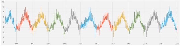
Microsoft’s AI for earth project (Figure 1) looks at the application of streaming data from sources such as satellites to do land cover analysis, sensors on and above farm land to improve agriculture outcomes and crowd sourced data to help understand biodiversity.

Figure 1. Applications of streaming include land cover analysis, using sensor data for improving agriculture and biodiversity. From https://www.microsoft.com/en-us/aiforearth
The internet of things is exploding with sensor data as are on-line experiments of all types. This data will be aggregated in edge computing networks that do initial analysis with results fed to the cloud systems for further analysis. Urban Informatics is a topic that has emerged as critical to the survival of our cities and the people who live in them. Sensors of all types are being deployed in cities to help understand traffic flow, microclimates, local pollution and energy waste. Taken together this sensor data can paint a portrait of the city that planners can use to guide its future. Streaming data and edge computing is a topic that will involve the growing capabilities and architecture of the cloud. We will return to this later in this document.
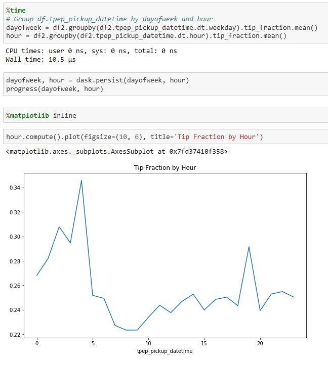
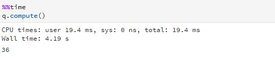
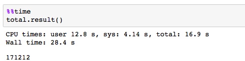
Interactive big data exploration
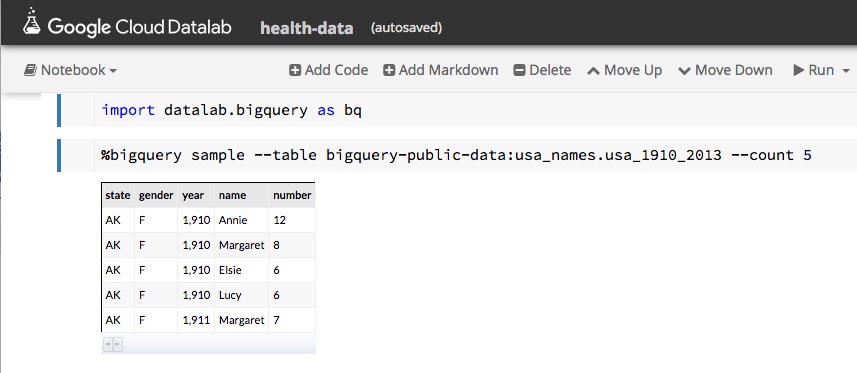
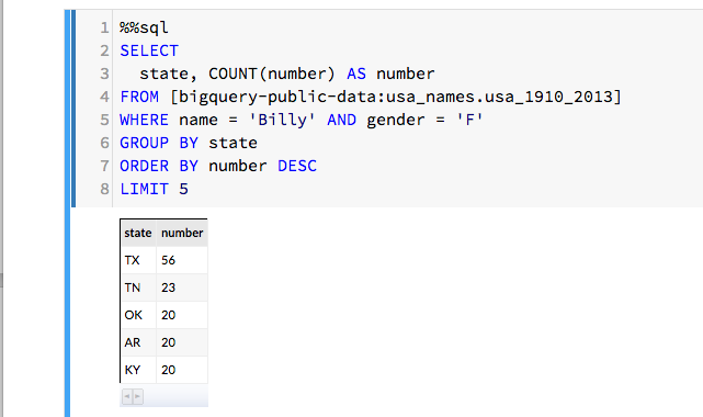
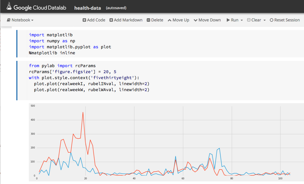
Being able explore and interact with data is a critical component of science. If it fits on our laptop we can use tools like Matlab, Excel or Mathematica to conduct small computational experiments and visualize the results. If the data is too big it must be stored on something bigger than that laptop. Traditional supercomputers are up to the task of doing the analysis, but because they are designed around batch computing there are not well suited to interactive use. The cloud exists to host services that can be used by thousands of simultaneous users. In addition, there is a new generation of interactive data analysis tools that are cloud-ready for use on very large data collections. This collection of tools includes Spark and Python Dask. In both cases these tools can be driven by the open-source Jupyter studio which provides a powerful, interactive compute and visualization tool. The commercial providers have adapted Jupyter and its interactive computational model into their offerings. Google has Cloud Datalab (Figure 2), Amazon uses Jupyter with its SageMaker Machine Learning platform and Microsoft provide a special data science virtual machine that runs Jupyter Hub so that teams of users can collaborate.
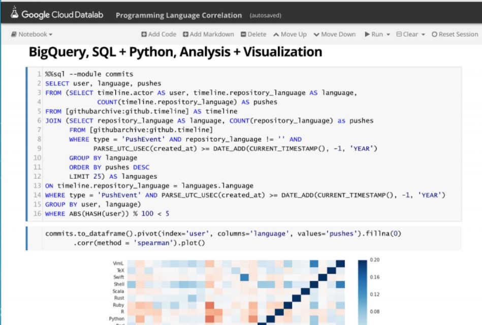
Figure 2. Google’s Cloud Data lab integrates SQL-like queries to be combined with Python code and visualization to a Jupyter based web interface. https://cloud.google.com/datalab/
Being able to interact with data at scale is part of the power of the cloud. As this capability is combined with advanced cloud hosted machine learning tools and other services, some very promising possibilities arise.
The quest for AI and an intelligent assistant for research
The commercial clouds were originally built to host web search engines. Improving those search engines led to a greater engagement of the tech companies with machine learning. That work led to deep learning which enabled machine language translation, remarkably strong spoken language recognition and generation and image analysis with object recognition. Many of these capabilities rival humans in accuracy and speed. AI is now the holy grail for the tech industry.
One outcome of this has been the proliferation of voice-driven digital assistants such as Amazon’s Echo, Microsoft’s Cortana, Apple’s Siri and Google Assistant. When first introduce these were novelties, but as they have improved their ability to give us local information, do web searching, keep our calendars has improved considerably. I believe there is an opportunity for science here.
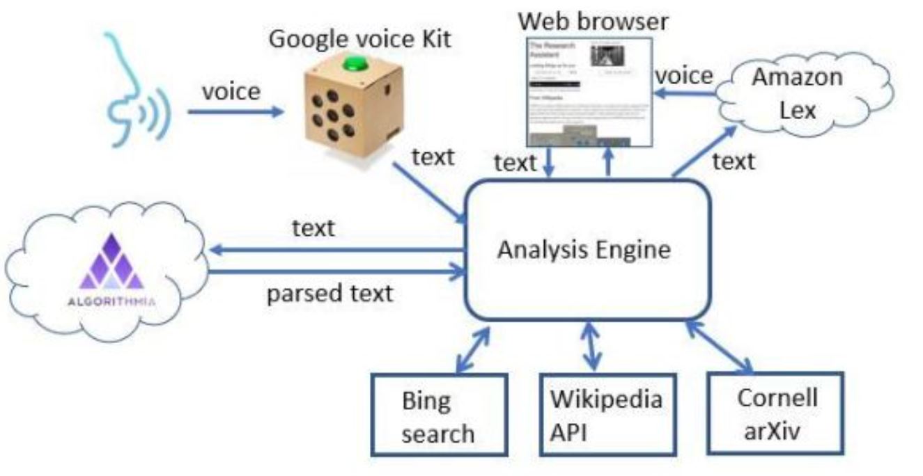
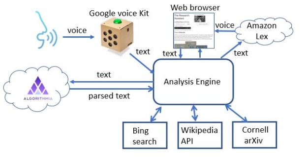
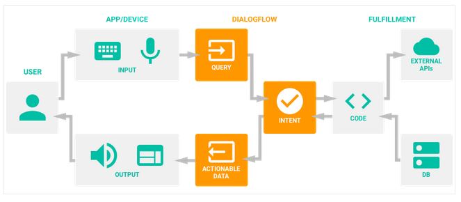
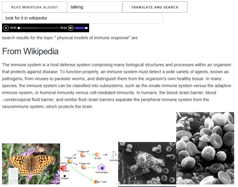
Ask the question “what would it take to make Alexa or Cortana help with my research?” The following use cases come to mind.
- Provide a fast and accurate search of the scientific literature for a given specific scientific concept or topic and not just a keyword or specific author. Then ask who is working on or has worked on this topic? Is there public data in the cloud related to experiments involving this topic? Translate and transcribe related audio and video.
- Understand and track the context of your projects.
- Help formulate, launch and monitor data analysis workflows. Then coordinate and catalog results. If state-space search is involved, automatically narrow the search based on promising findings.
- Coordinate meetings and results from collaborators.
If I ask Alexa to do any of this now, she would politely say “Sorry. I can’t help you with that.” But with the current rate of change in cloud AI tools, ten years seems like a reasonable timeframe.
Figure 3. Siri’s science geek grandson.
Technical Revolutions in the Cloud
Two of the three scenarios above are here now or very close. The third is some ways off. There have been three major changes in cloud technology in the past five years and some aspects of these changes are true game-changers for the industry. The first, and most obvious is the change in scale of cloud deployments. The two leaders, AWS and Azure are planetary in scale. This is illustrated in Figure 4 below.
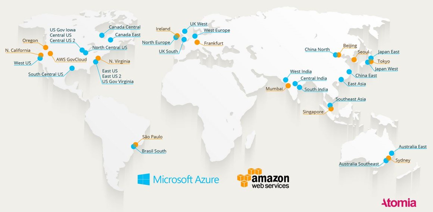
Figure 4. A 2016 map of cloud coverage from Atomia.com. https://www.atomia.com/2016/11/24/ comparing-the-geographical-coverage-of-aws-azure-and-google-cloud/ There is some inaccuracy here because AWS and Azure define regional data centers differently, so counting the dots is not a good comparison. In addition, data centers are now under construction in South Africa and the Middle East.
This map does not include all the data centers run by the smaller cloud providers.
Cloud Services
A major departure from the early days of the cloud, where scientists focused on storage and servers, has been an explosion in pay-by-the-hour cloud hosted services. In addition to basic IaaS the types of services available now are:
- App services: Basic web hosting, mobile app backend
- Streaming data: IoT data streams, web log streams, instruments
- Security services: user authentication, delegation of authorization, privacy, etc.
- Analytics: database, BI, app optimization, stream analytics
- Integrative: networking, management services, automation
In addition, the hottest new services are AI machine learning services for mapping, image classification, voice-to-text and text-to-voice services and text semantic analysis. Tools to build and train voice activated bots are also now widely available. We will take a look at two examples.
A planet scale database
The Azure Cosmos DB is a database platform that is globally distributed. Of course, distributing data across international boundaries is a sensitive topic, so the Cosmos platform allows the database creator to pick the exact locations you want copies to reside. When you create an instance of the database you use a map of Azure data centers and select the locations as shown in Figure 5.

Figure 5. Cosmos DB. A database created in central US and replicated in Europe, South India and Brazil.
The database can support 4 modes: Documents, key-value Graph and NoSQL. In addition, there are five different consistency models the user can select: eventual, consistent prefix, session, bounded stateless and strong consistency all with 99.9% guarantee of less than 15ms latency. My own experiments validated many these claims.
Cloud AI Services
The commercial clouds are in a race to see who can provide the most interesting and useful AI services on their cloud platform. This work began in the research laboratories in universities and companies over the past 25 years, but the big breakthroughs came when deep learning models trained on massive data collections began to reach levels of human accuracy. For some time now, the public cloud companies have provided custom virtual machines that make it easy for technically sophisticated customers to use state of the art ML and neural network tools like TensorFlow, CNTK and others. But the real competition is now to provide services for building smart applications that can be used by developers lacking advanced training in machine learning and AI. We now have speech recognition, language translation, image recognition capabilities that can be easily integrated into web and mobile applications.
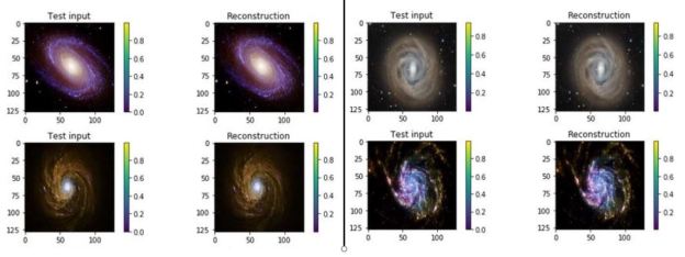
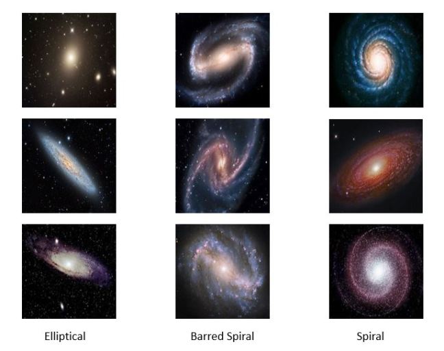
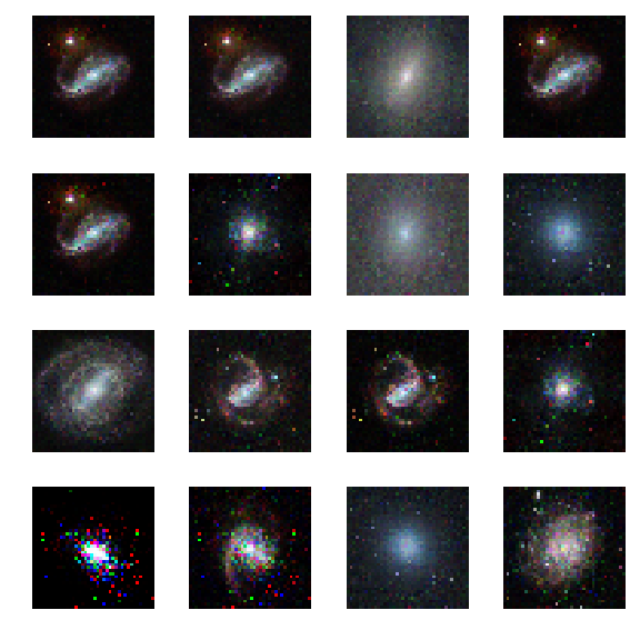
We gave this a try with services that use a technique called Transfer Learning to make it possible to re-train a deep neural network to recognize objects from a narrow category using a very small training set. We chose images of galaxies and used the services of IBM Watson, Azure and Amazon. Figure 6 illustrates the results from IBM’s tool. The results were surprisingly good.
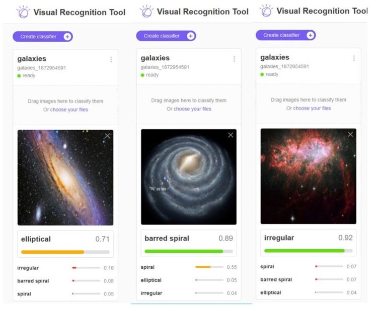
Figure 6. IBM’s Watson recognizing previously unseen images of three different galaxies. The details of this study are here: https://esciencegroup.wordpress.com/2018/02/16/cloud-services-for-transfer-learning-on-deep-neural-networks/
The Revolution in Cloud Service Design
Making all of these services work, perform reliably and scale to thousands of concurrent users forced a revolution in cloud software design. In order to support these applications, the tech companies needed a way to design them so that they could be scaled rapidly and updated easily. They settled on a design pattern that based on the idea of breaking the applications into small stateless components with well defined interfaces. Statelessness meant that a component could be replaced easily if it crashed or needed to be upgraded. Of course, not everything can be stateless, so state is saved in cloud hosted databases. Each component was a “microservice” and it could be built from containers or functions. This design pattern is now referred to as “cloud native” design. Applications built and managed this way include Netflix, Amazon, Facebook, Twitter, Google Docs, Azure CosmosDB, Azure Event hub, Cortana, Uber.
 Figure 7. Conceptual view of microservices as stateless services communicating with each other and saving needed state in distribute databases or tables.
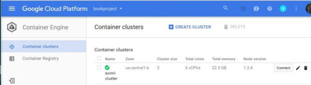
To manage applications that required dozens to hundreds of concurrently running microservice you need a software foundation or container orchestration system to monitor the services and schedule them on available resources. Several candidates emerged and are used. Siri, for example, is composed of thousands of microservices running on the Apache Mesos system. Recently cloud providers have settled on a de-facto standard container orchestrator built by Google and released as open source called Kubernetes. It is now extremely easy for any customer to use Kubernetes on many cloud deployments to launch and manage cloud native applications.
Serverless Functions
The next step in the cloud software evolution was the introduction of “serverless functions”. The original idea of cloud computing involved launching and managing a virtual machine. However, suppose you want to have a cloud-based application whose sole job is to wait for an event to trigger some action. For example, monitor a file directory and wait for a change such as the addition of a new file. When that happens, you want to send email to a set of users alerting them of the change. If this is a rare event, you don’t want to have to pay for an idle virtual machine that is polling some service looking for a change. Amazon was the first to introduce the concept of a function-as-a-service. With AWS Lambda, you only need to describe the function in terms of the trigger event and the output actions it takes when the even appears. As illustrated in Figure 8, there are many possible triggers and corresponding output channels.
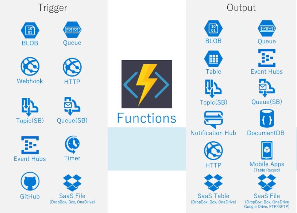
Figure 8. From Amazon AWS. The triggers and outputs of a lambda function.
In addition to AWS Lambda, Azure Functions, Google Functions, IBM OpenWhisk are similar systems. OpenWhisk is now open source. Another open source solution is Kubeless that allow you to deploy a lambda-like system on top of your Kubernetes cluster. These serverless systems let you scale up and down extremely rapidly and automatically. You can have hundreds of instances responding to events at once. And the cost is based on charge-by-use models. AWS has introduced AWS Fargate which allows any containerized application to run in serverless mode.
The Edge and the Fog
The frontier of cloud computing is now at the edge of the network. This has long been the home of content distribution systems where content can be cached and access quickly, but now that the Internet-of-Things (IoT) is upon us, it is increasingly important to do some computing at the edge. For example, if you have a thousand tiny sensors in a sensitive environment or farm and you need to control water from sprinklers or detect severe weather conditions, it is necessary to gather the data, do some analysis and signal an action. If the sensors are all sending WIFI messages they may be routable to the cloud, but a more common solution is to provide local computing that can do some event preprocessing and response while forwarding summary data to the cloud. That local computing is called the Edge, or if a distributed systems of edge servers, the Fog.
If serverless functions are designed to respond to signals, that suggests that it should be possible to extend them to run in the edge servers rather than the cloud. AWS was the first to do this with a tool called GreenGrass that provides a special runtime system that allows us to push/migrate lambda functions or microservices from the data center to the edge. More recently Microsoft has introduced Azure IoT Edge which is built on open container technologies. Using an instance open source Virtual Kubelet deployed on the edge devices we can run our Kubernetes containers to run on the edge. You can think of a Kubelet as the part of Kubernetes that runs on a single node. This enables Kubernetes clusters to span across the cloud and edge as illustrated in Figure 9.

Figure 9. shows a sketch of migrating containerized functions to edge function. That way our IOT devices can communicate with locally deployed microservices. These microservices can communicate with cloud-based services. The edge function containers can also be updated and replaced remotely like any other microservice.
The Evolution of the Data Center
As mentioned at the beginning of this paper, the early days (2005) of cloud data center design systems were based on very simple server and networks were designed for outgoing internet traffic and not bisectional bandwidth for parallel computing. However, by 2008 interest in performance began to grow. Special InfiniBand sub-networks were being installed at some data centers. The conventional dual-core servers were being replaced by systems with up to 48 cores and multiple GPU accelerators. By 2011 most of the commercial clouds and a few research clouds had replaced traditional network with software defined networking. To address the demand of some of its customers, in 2017 Microsoft added Cray® XC™ and Cray CS™ supercomputers to a few data centers and then acquired the company cycle computing.
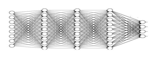
From 2016 we have seen progress focused on performance and parallelism. The driver of this activity has been AI and, more specifically, the deep neural networks (DNNs) driving all the new services. There are many types of DNNs but two of the most common are convolutional, which look like a linear sequence of special filters, and recurrent networks which, as the name implies, are networks with a feedback component. And there are two phases to neural network design and use. The first is the training phase which requires often massive parallelism and time. But it is usually an off-line activity. The second phase is called inference and it refers to the activity of evaluating the trained network on classification candidates. In both the convolutional and recurrent network inference boils down to doing a very large number of matrix-vector and matrix-matrix multiplies where the coefficients of the matrix are the trained model and the vector represent the classification candidates. To deliver the performance at scale that was needed by the AI services it was essential to do these operations fast. While GPUs were good, more speed was needed.
Google’s Tensor Processing Unit
In 2015 Google introduced the Tensor Processing Unit (TPU) and the TPU2 in 2017.
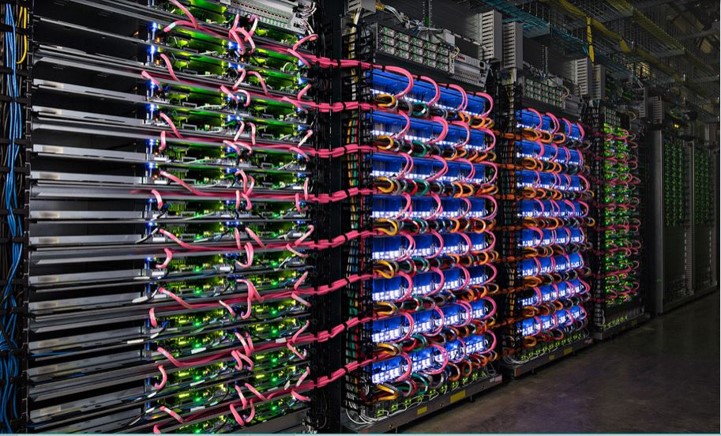
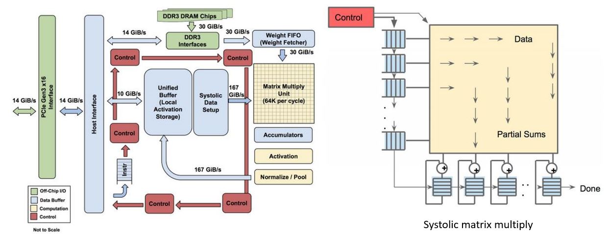
Figure 10. Above, Google data center. https://www.nextplatform.com/2017/05/22/hood-googles-tpu2-machine-learning-clusters/ Below architecture of Google Tensor Processing Unit TPU. From “In-Datacenter Performance Analysis of a Tensor Processing Unit”, Norman P. Jouppi et al. ISCA 2017 https://ai.google/research/pubs/pub46078
Figure 10 illustrates several racks of TPU equipped servers and the functional diagram of the TPU. One of the key components is the 8-bit matrix multiply capable of delivering 92 TeraOps/second (TOPS). (It should be noted that DNNs can be well trained on less than IEEE standard floating-point standards and floating point systems with small mantissa are popular.) The multiply unit uses a systolic algorithm like those proposed for VLSI chips in the 1980s.
Microsoft’s Brainwave
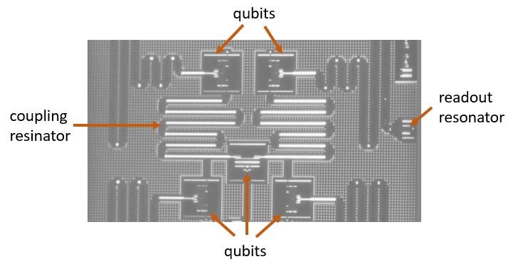
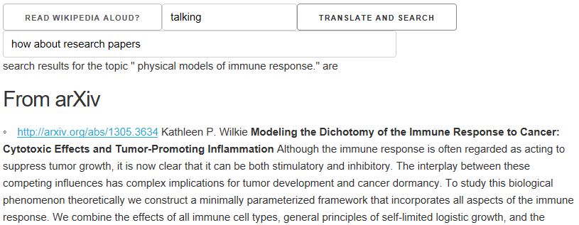
In 2011 a small team in Microsoft Research led by Doug Burger began looking at the use of FPGAs to accelerate the search result ranking produced by Bing. Over several iterations they arrived at a remarkable design that allowed them to put the FPGA between the network and the NIC so that the FPGA could be configured into separate plane of computation that can be managed and used independently from the CPU (see Figure 11). Used in this way groups of FPGAs could be configured into a subnetwork to handle tasks such as, database queries and inference stage of deep learning in addition to Bing query optimization.
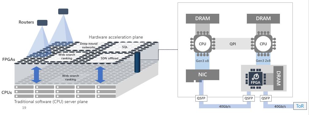
Figure 11. The Brainwave architecture.

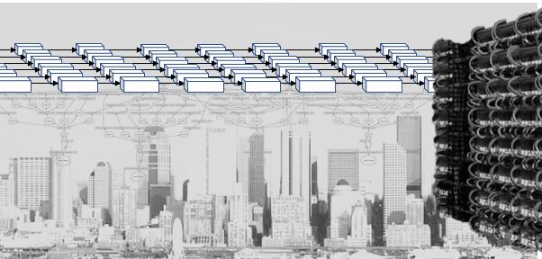
Figure 12. The brainwave software stack for mapping a DNN to one or more FPGAs. From BrainWave_HOTCHIPS2017.pptx, Eric Chung, et. al., https://vneetop.wordpress.com/ 2017/10/28/accelerating-persistent-neural-networks-at-datacenter-scale/
The team also built a software stack that could really make this possibility a reality. What makes much of this possible is that the models for DNNs are all based on flow graphs which describe sequences of tensor operations. As shown in Figure 12 above, the flow graphs can be compiled to a graph internal representation that can be split and partitioned across one or more FPGAs. They refer to the result as a hardware microservice. Just recently Mary Wall [see endnote 2] wrote a nice blog about the teams work on using this idea to do deep learning inference on land cover maps. Each compiled inference hardware microservice is mapped to a single FPGA, but they used 800 of the inference instances in parallel with 80 VMs to process 20 terabytes of aerial imagery into land cover data for the entire United States. It took only about 10 minutes for a total cost of $42. [see endnote3] Mary Wall’s code is in the blog and available in Github.
Conclusion
Cloud data centers are getting high performance networks (with latencies of only a few microseconds in the case of Azure Brainwave) and immense computing capacity such as the tensor processing capability of Google’s TPU. At the same time designers of supercomputers are having to deal with more failure resilience and complexity in the design of the first exascale supercomputers. For the next generation exascale systems the nodes will be variations on a theme of multicore and GPU-style accelerators.
Observed from a distance, one might conclude the architectures of cloud data centers and the next generation of supercomputers are converging. However, it is important to keep in mind that the two are designed for different purposes. The cloud is optimized for fast response for services supporting many concurrent globally distributed clients. Supers are optimized for exceptionally fast execution of programs on behalf of a small number of concurrent users. However, it may be the case that an exascale system may be so large that parts of it can run many smaller parallel jobs at once. Projects like Singularity provide a solution for running containerized application on supercomputers in a manner similar to the way microservices are run on a cloud.
Possible Futures
The continuum: edge+cloud+supercomputer
There are interesting studies showing how supercomputers are very good at training very large, deep neural networks. Specifically, NERSC scientists have show the importance of this capability in many science applications[4]. However, if you need to perform inference on models that are streamed from the edge you need the type of edge+cloud strategy described here. It not hard to imagine scenarios where vast numbers of instrument streams are handled by the edge and fed to inference models on the cloud and those models are being continuously improved on a back-end supercomputer.
A data garden
In the near future, the most important contribution clouds can make to science is to provide access to important public data collections. There is already reasonable start. AWS has an opendata registry that has 57 data sets covering topics ranging from astronomy to genomics. Microsoft Research has a Data Science for Research portal with a curated collection of datasets relating to human computer interaction, data mining, geospatial, natural language processing and more. Google cloud has a large collection of public genomics datasets. The US NIH has launch three new cloud data and analytics projects. They include the Cancer Genomics Cloud led by the Institute for Systems Biology with Google’s cloud, FireCloud from the Broad Institute also using Google’s cloud and Cancer Genomics Cloud (CGC), powered by Seven Bridges. These NIH facilities also provide analytics frameworks designed to help research access and effective use the resources.
I am often asked about research challenges in cloud computing that student may wish to undertake. There are many. The fact that the IEEE cloud computing conference being held in San Francisco in July received nearly 300 submissions shows that the field is extremely active. I find the following topics very interesting.
- Find new ways to extract knowledge from the growing cloud data garden. This is a big challenge because the data is so heterogeneous and discovery of the right tool to use to explore it requires expert knowledge. Can we capture that community knowledge so that non-experts can find their way? What are the right tools to facility collaborative data exploration?
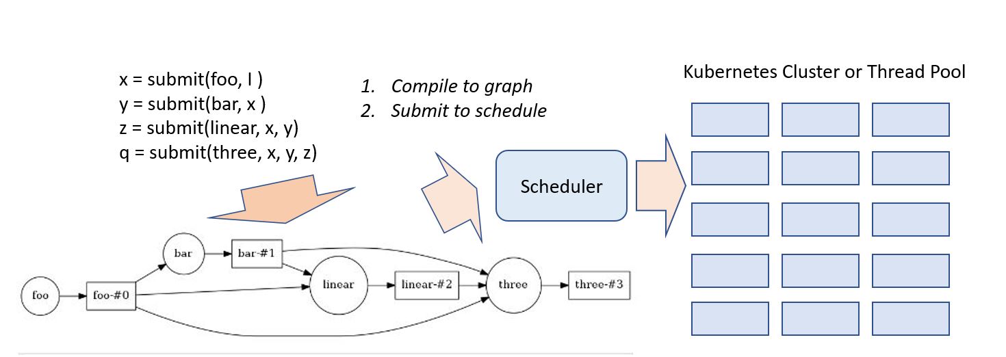
- There are enormous opportunities for systems research in the edge-to-cloud-to-supercomputer path. How does one create a system to manage and optimize workflows of activities that span this continuum? Is there a good programming model for describing computations involving the edge and the cloud? Can a program be automatically decomposed into the parts that are best run on the edge and the parts on cloud? Can such a decomposition be dynamically adjusted to account for load, bandwidth constraints, etc.?
- Concerning the intelligent assistant for research, there are a number of reasonable projects short of build the entire thing. Some may be low hanging fruit, and some may be very hard. For example, ArXiv, Wikipedia and Google search and Bing are great for discovery but in different ways. Handling complex queries like “what is the role of quantum entanglement in the design of a quantum computer?” should lead to a summary of the answer with links. There is a lot of research on summarization and there are a lot of sources of data. Another type of query is “How can I access data on genetic indicators related to ALS?” Google will go in the right direction, but it takes more digging to find data.
These are rather broad topics, but progress on even the smallest part may be fun.
[1] L. Ramakrishnan, P. T. Zbiegel, S. Campbell, R. Bradshaw, R. S. Canon, S. Coghlan, I. Sakrejda, N. Desai, T. Declerck, and A. Liu. Magellan: Experiences from a science cloud. In 2nd International Workshop on Scientific Cloud Computing, pages49–58., ACM, 2011.
P. Mehrotra, J. Djomehri, S. Heistand, R. Hood, H. Jin, A. Lazanoff, S. Saini, and R. Biswas. Performance evaluation of Amazon EC2 for NASA HPC applications. In 3rd Workshop on Scientific Cloud Computing, pages 41–50. ACM, 2012
[2] https://blogs.technet.microsoft.com/machinelearning/2018/05/29/how-to-use-fpgas-for-deep-learning-inference-to-perform-land-cover-mapping-on-terabytes-of-aerial-images/ a blog by Mary Wall, Microsoft
[3] https://blogs.microsoft.com/green/2018/05/23/achievement-unlocked-nearly-200-million-images-into-a-national-land-cover-map-in-about-10-minutes/ from Lucas Joppa – Chief Environmental Scientist, Microsoft
[4] https://www.hpcwire.com/2018/03/19/deep-learning-at-15-pflops-enables-training-for-extreme-weather-identification-at-scale/


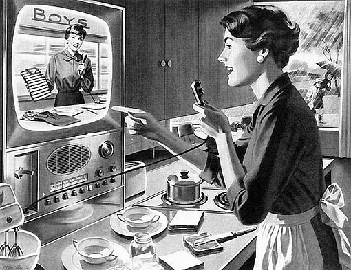


 Fig 5. Microsoft FPGA based Project Brainwave [4, 5]
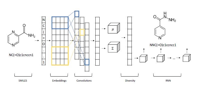


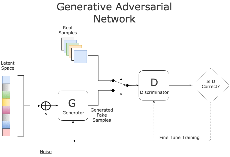
 into so that they look like they come from the distribution
  for our collection c. Think of it as a function
![Disc: R^m \to [0,1]](https://s0.wp.com/latex.php?latex=+Disc%3A+R%5Em+%5Cto+%5B0%2C1%5D+&bg=ffffff&fg=444444&s=0&c=20201002)
 is probability that X is in the collection c. To make this more “discriminating” let us also insist that
  . In other word, the discriminator is designed to discriminate between the real c objects and the generated ones. Of course, if the Generator is really doing a good job of imitating


