

Abstract.
This brief note is intended to illustrate why the programming language Julia is so interesting to a growing number of computational and data scientists. Julia is designed to deliver high performance on modern hardware while retaining the interactive capabilities that make it well suited for Jupyter-style scientific exploration. This paper illustrates, with some very unscientific examples, how Julia can be deployed and with Docker and Kubernetes in the cloud.
Introduction
In all our previous posts we have used Python to build applications that interact with cloud services. We used Python because everybody knows it. However, as many scientists have now discovered, for scientific applications the programming language Julia is a better alternative. This note is not a Julia tutorial, but rather, it is intended to illustrate why Julia is so interesting. Julia was launched in 2012 by Jeff Bezanson, Stefan Karpinski, Viral B. Shah, and Alan Edelman and is now gaining a growing collection of users in the science community. There is a great deal of Julia online material and a few books (and some of it is up to date). In a previous blog post we looked at Python Dask for distributed computing in the cloud. In this article we focus on how Julia can be used for those same parallel and distributed computing tasks in the Cloud. Before we get to the cloud some motivational background is in order.
1. Julia is Fast!
There is no reason a language for scientific computing must be as dull as Fortran or C. Languages with lots of features like Java, Python and Scala are a pleasure to use but they are slow. Julia is dynamic (meaning it can run in a read-eval-print-loop in Jupyter and other interactive environments), it has a type system that support parametric polymorphism and multiple dispatch. It is also garbage collected and extremely extensible. It has a powerful package system, macro facilities and a growing collection of libraries. It can call C and Python directly if it is needed.
And it generates fast code. Julia uses a just-in-time compiler that optimized your program depending on how you use it. To illustrate this point, consider a simple function of the form
function addem(x)
   # do some simple math with x
   x += x*x
return x
end
Because we have not specified the exact type of x, this defines a generic function: it will work with arguments of any type that has meaning for the math operations used. But when we invoke it with a specific type, such as int or float, a version of the function is compiled on the fly that is specialized to that type. This specialization takes a bit of time, but when we invoke the function a second time with that argument type, we used the specialized version. As illustrated in Figure 1, we called the function twice with integer arguments. The second call is substantially faster than the first. Calling it with a floating point argument is slow until the specialized version for floating point variables is created, then the function runs fast.
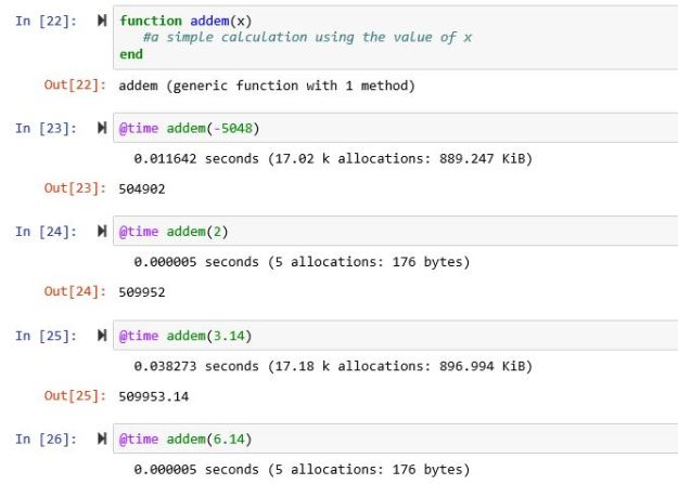
Figure 1. Using a timing macro to measure the speed of function calls. In step 23 the generic version is called with an integer. The second call uses the version optimized for integers. In steps 25 an 26 the specialized version for floating point numbers is generated and run.
The Julia team has put together a benchmark set of small examples written in several languages. We extracted the benchmarks for C, Python and Julia and ran them. The resulting execution time are shown below. As you can see, the Julia code generation is arguably as good as C (compiled with optimized gcc). Relative to Python it is as much as 50 times faster. Figure 2 makes this more explicit. The only benchmark where Python is within a factor of two is matrix multiply and that is because Python is using the optimized numpy.linalg libraries.
| Benchmark | python | gcc – O | julia |
| recursion_fibonacci | 2.977 | 0.000 | 0.037 |
| parse_integers | 2.006 | 0.117 | 0.197 |
| userfunc_mandelbrot | 6.294 | 0.068 | 0.065 |
| recursion_quicksort | 12.284 | 0.363 | 0.364 |
| iteration_pi_sum | 558.068 | 22.604 | 22.802 |
| matrix_statistics | 82.952 | 11.200 | 10.431 |
| matrix_multiply | 70.496 | 41.561 | 41.322 |
| print_to_file | 72.481 | 17.466 | 8.100 |
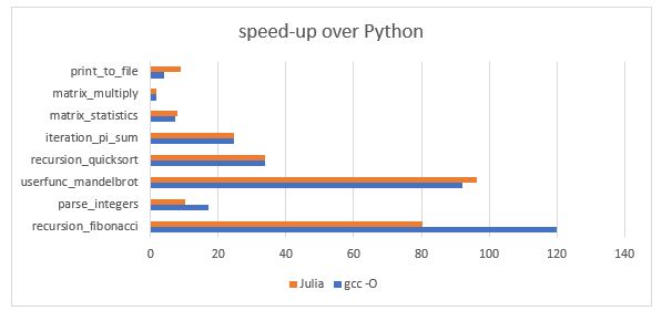
Figure 2. Speed-up of Julia and C relative to Python
2. Julia Math and Libraries
Doing basic linear algebra and matrix computation in Julia is trivial. The following operations each take less than one second in Jupyter using the package LinearAlgebra.jl.
M = rand(1000, 1000); # generates a 1000 by 1000 matrix of random floats
N = M^-1 # compute the inverse of M
C = M*M’ # M’ is the transpose so the product is symmetric.
Q = svd(C) # computes the singular value decomposition of C.
Q.S # are the singular values.
Sparse matrices are also supported along with a large number of other matrix creation and manipulation operations.
Differential Equations
The differential equation package built by a team led by Christopher Rackauckas is one of the most impressive. To illustrate this we consider an example from their excellent tutorial. The Lorenz attractor is a fascinating example of a chaotic solution to a system of differential equations that model convection. The system involves the evolution in 3D of a system that is characterized by three parameters. As shown below the equations are expressed exactly as you would describe them mathematically (dx is dx/dt) and the three parameters ar sigma, rho and beta. The initial point is (1,0,0) and the region is integrated over [0,100]. The package automatically picks an appropriate solver and the output is plotted as shown in Figure 3. Running this on a Mac mini took about 5 seconds. We used another package “Plots” to render the image.
g = @ode_def LorenzExample begin
dx = σ*(y-x)
dy = x*(ρ-z) – y
dz = x*y – β*z
end σ ρ β
u0 = [1.0;0.0;0.0]
tspan = (0.0,100.0)
p = [10.0,28.0,8/3]
prob = ODEProblem(g,u0,tspan,p)
sol = solve(prob)
plot(sol)
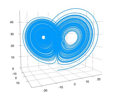
Figure 3. Plot of the Lorenz attractor solution. (yes, Greek Unicode character names are valid.)
Note: Thomas Breloff provides a more explicit integration with a Gif animation in this Plots tutorial. As with the above example, Breloff’s solution works well in Jupyter.
Julia Distributed Computing in the Cloud
Julia has several packages that support parallel computing. These include a library for CUDA programming, OpenMP, Spark and MPI.jl for MPI programming. MPI is clearly the most reliably scalable parallel computing model for tasks involving 10000 or more cores. It is based on low-latency, two-sided communication in which coordinated, synchronized send-receive pairs and collective operations are executed in parallel across large clusters equipped with specialized networking. While Julia can be used with MPI, the natural model of communication in Julia is based on one-sided communication based on threads, tasks, futures and channels. We will use the package Distributed.jl to demonstrate this.
The Julia distributed computing model is based on distributing tasks and arrays to a pool of workers. Worker are either Julia processes running on the current host or on other hosts in your cluster. (In the paragraphs that follow we show how to launch local workers, then workers on other VMs in the cloud and finally workers as docker containers running in a Kubernetes cluster.
Let’s begin with a trivial example. Create a function which will flip a coin “n” times and count the number of heads.
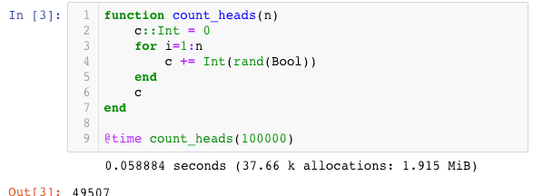
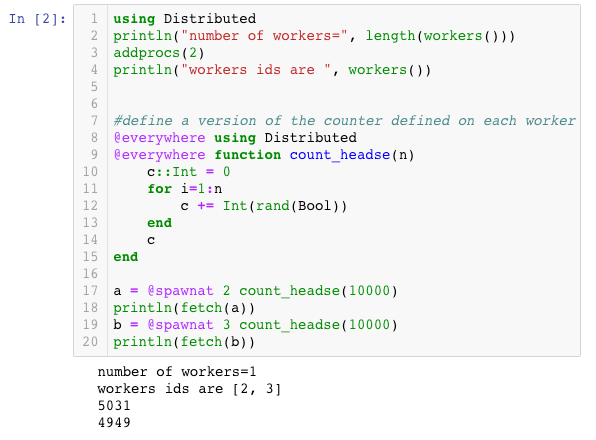
Here we generated random Boolean values and converted them to 0 or 1 and added them up. Now let’s add some workers.
First we include the “Distributed” package and count the current number of workers. Next using the “addproc( )” function we added two new worker processes on the same server running this Jupyter notebook. Workers that our notebook process knows about are identified with an integer and we can list them. (The notebook process, called here the master, is not a worker)
The worker processes are running Julia but they don’t know about the things we have defined in the master process. Julia has a very impressive macro facility that is used extensively in the distributed computing package to distributed code objects to the workers and to launch remote computations.
When we create a function in the master that we want executed in the workers we must make sure it also gets defined in that worker. We use the “@everywhere” macro to make sure things we define locally are also defined in each worker. We even must tell the workers we are using the Distributed package. In the code below we created a new version of our count_heads function and distributed it.
Julia uses the concept of futures to launch computation on the workers. The “@spawnat” macro takes two parameters: the ID of a worker and a computation to be launched. What is returned is a future: a placeholder for the final result. By “fetch( a)” we can grab the result of the future computation and return it to our calling environment. (Some library functions like “printf()” when executed on the workers are automatically mapped back to the master.)
In the following example we create two local workers and define a function for them to execute. Workers each have a unique integer ID and we print them. Then we use @spawnat to launch the function on each worker in turn.
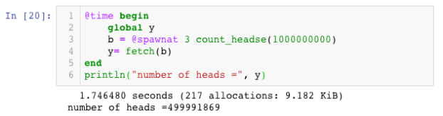
We can easily measure the cost of this remote function evaluation with the @time macro as follows. We enclose the call and fetch in a block and time the block. (Notice we have increased the number of coins to 109 from 104.)
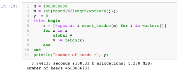
If we want both workers working together, we can compose a list of spawned invocations with a construct of the form
[ @spawn at i expr(i) for i in range]
This returns a list (technically, in Julia it is an array) of futures. We can then grab the result of each future in turn. The result is shown below. This is run on a dual core desktop machine, so parallelism is limited but, in this case, the parallel version is 1.85 times faster than the individual call. The reason that it is not exactly two time faster is partly due to the overhead in sequentially launching and resolving the futures. But it is also due to communication delays and other OS scheduling delays.
A more compact and elegant way to write this parallel program is to use the Julia distributed parallel map function pmap(f, args). pmap takes a function and applies it to each element of a set of arguments and uses the available workers to do the work. The results are returned in an array.
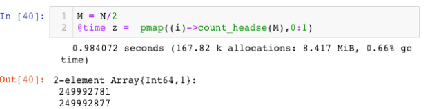
In this case count_headse did not need an argument so we constructed an anonymous function with one parameter to provide to the pmap function. In this execution we were only concerned with dividing the work into two parts and then letting the system schedule and execute them with the available worker resources. We chose 2 parts because we know there is two workers. However, we could have divided into 10 parts and applied 10 argument values and the task would have been accomplished using the available workers.
Julia distributed across multiple host machines.
To create a worker instance on another host Julia uses secure shell (ssh) tunnels to talk to it. Hence you need five things: the IP address of the host, the port that secure shell uses, the identity of the “user” on that host and the private ssh key for that user. The ssh key pair must be password-less. The location of the Julia command on that host is also needed.
In this and the next example we simplify the task of deploying Julia on the remote host by deploying our Julia package as a docker container launched on that host. To make the ssh connection work we have mapped the ssh port 22 on the docker container to port 3456 on the host. (We describe the container construction and how it is launched in the next section.)
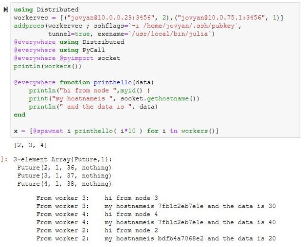
In the previous section we provided “addprocs()” with a single integer representing the number of worker we wanted launched locally. As shown below, the remote version requires a bit more. We supply an array of tuples to addprocs() where each tuple provides the contact point and the number of workers we want there. In this example we spawn 2 workers on one remote node and one worker on the other. We also provide the local location of the private key (here called pubkey) in the sshflags argument.
We also want each worker to have the Distributed.jl package and another package called “PyCall” which enables calling python library functions. We demonstrate the python call with a call to socket.hostname() in each worker. Notice that the remote function invocation returns the “print” output to the master process. The strange hostnames that are printed are the synthetic host names from the docker containers.
This example did not address performance. We treat that subject briefly at the end of the next section.
Channels
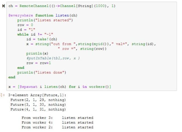
In addition to spawning remote tasks Julia supports a remote channel mechanism. This allows you to declare a channel that can carry messages of a given type and hold them for remote listeners to pickup. In the example below we declare a remote channel that carries string messages and a function defined for the listeners to use. The worker can use the “take!()” function to remove an item from the channel and the master uses “put!()” to fill the channel. The message “-1” tells the listener to stop listening.
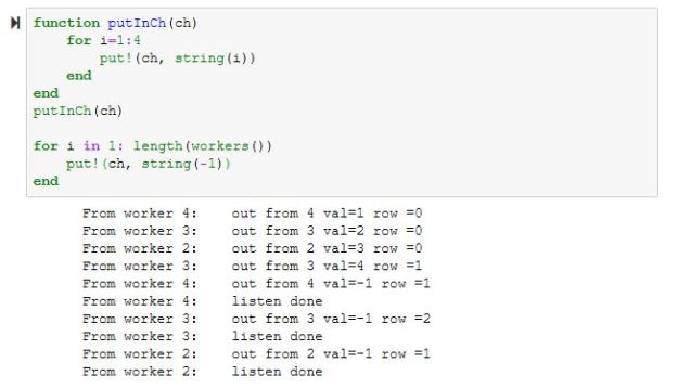
Using the channel mechanism one can use Julia to have a group of workers respond to a queue of incoming messages. In the Github site for this post we have put an example where the workers take the channel messages and put the results into an Azure table.
Julia Distributed Computing on Kubernetes
Depending upon your favorite flavor of cloud there are usually three or four ways to spin up a cluster of nodes to run a distributed computation. The most basic way to do this is to launch a group of virtual machines where each has the needed resources for the problem you want to solve. For Julia, the best thing to do is launch instances of a ‘data science VM” that is available on AWS or Azure. There are two things your VM needs: an installation of Julia version 1.0.0 or later and the ability to ssh to it without using a password.
Here is how to do this on Azure. First, run “ssh-keygen” and it will step you through the process of generating a key-pair and give you the option of having no password. Then from the Azure portal select “create a resource” and search for Linux data science VM. As you go through the installation process when it asks for a key, paste in the public key you just generated. When the VM is up you can ssh to it to verify that it has the needed version of Julia installed by typing “Julia” at the command line. If it can’t find Julia you will need to download and install it. While you are logged and running Julia, you should also install some of the libraries your distributed program will need. For example, Distributed.jl and PyCall.jl or any package specific to your application. If you have a large cluster of VMs, this is obviously time consuming.
A better solution is to package your worker as a Docker container and then use Kubernetes to manage the scale-out step. We have set up a docker container dbgannon/juliacloud2 in the docker hub that was be used for the following experiments. This container is based on Jupyter/datascience-notebook so it has a version of Jupyter and Julia 1.0.0 already installed. However to make it work has a Julia distributed worker it must be running the OpenSsh daemon sshd. A passwordless key pair has been preloaded into the appropriate ssh directory. We have also installed the Jullia libraries Distributed.jl, PyCall.jl and IJulia.jl. PyCall is needed because we need to call some python libraries and Ijulia.jl is critical for running Julia in Jupyter. We have included all the files needed to build and test this container in Github.
Launching the container directly on your local network
The docker command to launch the container on your local network is
docker run -it -d -p 3456:22 -p 8888:8888 dbgannon/juliacloud2
This exposes the ssh daemon on port 3456 and, if you run the jupyter notebook that is on port 8888. To connect to the server you will need the ssh key which is found on the Github site. (If you wish to use your own passwordless keypair you will need to rebuild the docker container using the files in Github. Just replace pubkey and pubkey.pub. and rebuild the container.) To connect to the container and start Jupyter use the key pubkey.
ssh -i pubkey jovyan@localhost -p 3456
…
jovyan@bdfb4a7068e2:$ jupyter notebook
Notice that when you did this you were prompted to agree to add the ECDSA key fingerprint to your known hosts file. Jupyter will come up on your local machine at http://localhost:8888 and the password is “julia”. If you are running this remotely replace localhost with the appropriate IP and make sure port 8888 is open. To launch worker instances run docker as above (but you don’t need “-p 8888:8888”. ) When they are up you will need to ssh to each from your instance running jupyter. Doing this step is necessary to put the ECDSA key into the known hosts of your master jupyter instance.
Launching the containers from Kubernetes
Now that Kubernetes has become a cloud standard it is relatively easy to create a cluster from the web portal. The experiments here were completed on a small 5 node cluster of dual core servers. Once the cluster was up it was easy to launch the individual components from the Kubernetes command line. Creating the Jupyter controller required two commands: the first to create the deployment and the second to expose it through a load balancer as a service.
kubectl run jupyter --image=dbgannon/jupyter --port=8888
kubectl expose deployment jupyter --type=LoadBalancer
Creating the worker deployment required one line.
kubectl run julcloud --image=dbgannon/juliacloud
(Note: this wad done with earlier versions of the Docker containers. Juliacloud2 described above combines the capabilities of both in one container.)
One the two deployments were running, we used the Kubernetes web portal to scale the julcloud deployment to 5 different pods as shown in Figure 4 below.
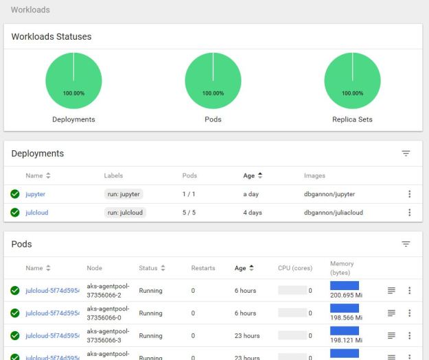
Figure 4. Kubernetes deployment of 5 worker pods and the Jupyter pod.
Unfortunately, we still needed to find the Ip address of each pod (which can be found on the Kubernetes portal) and ssh to each from the Python controller to add them to the known hosts file there. (It should be possible to automate this step.) of Using this configuration we ran two experiments. In the first we created a simple standard Monte Carlo simulation to compute Pi and ran it by allocating 2 workers per Kubernetes worker pod. The code is shown below.
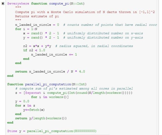
We scaled the number of pods to 10 and put two workers per pod and computed the speed up for N = 8*109 and N = 8*1010. The highly unscientific results are shown in the chart below. Notice that 10 pods and 20 workers is two workers per core, so we cannot realistically achieve speeds up much beyond 10, so a maximum speedup of 13.9 with 20 workers is good. ( In fact, it reflects likely inefficiency seen when run with only one worker.)
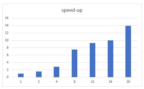
Figure 5. Speedup relative to one worker when using up to 20 workers and 10 pods on five servers.
The second experiment was to use 10 workers to pull data from a distributed channel and have them push it to the Azure table service. The source code for this experiment is in the Github repository.
Conclusion
There is a great deal that has not been covered here. One very important item missing from the above discussion is the Julia distributed array library. This is a very important topic, but judging from the documentation it may still be a bit of a work-in-progress. However I look forward to experimenting with it.
One of the applications of Julia that inspired me to take a closer look at Julia is the Celeste astronomy project that used 650,000 cores to reach petaflop performance at NERSC. Julia computing is now a company devoted to supporting Julia. Their website has many other great case studies.
There are many interesting Julia resources. Juliacon is an annual conference that brings together the user community. A brief look at the contents of the meeting videos (100 of them!) shows the diversity of Julia applications and technical directions.
