Google recently released a beta version of a new tool for data analysis using the cloud called Datalab. In the following paragraphs we take a brief look at it through some very simple examples. While there are many nice features of Datalab, the easiest way to describe it would be to say that it is a nice integration of the IPython Jupyter notebook system with Google’s BigQuery data warehouse. It also integrates standard IPython libraries such as graphics and scikit-learn and Google’s own machine learning toolkit TensorFlow.
To use it you will need a Google cloud account. The free account is sufficient if you are interested in just trying it out. You may ask, why do I need a Google account when I can use Jupyter, IPython and TensorFlow on my own resources? The answer is you can easily access BigQuery on non-trivial sized data collections directly from the notebook running on your laptop. To get started go to the Datalab home page. It will tell you that this is a beta version and give you two choices: you may either install the Datalab package locally on your machine or you may install it on a VM in the Google cloud. We prefer the local version because it saves your notebooks locally.
The Google public data sets that are hosted in the BigQuery warehouse are fun to explore. They include
- The names on all US social security cards for births after 1879. (The table rows contain only the year of birth, state, first name, gender and number as long as it is greater than 5. No social security numbers.),
- The New York City Taxi trips from 2009 to 2015,
- All stories and comments from “Hacker News”,
- The US Dept of Health weekly records of diseases reported from each city and state from 1888 to 2013,
- The public data from the HathiTrust and the Internet Book Archive,
- The global summary of the day’s (GSOD) weather from the national oceanographic and atmospheric administration from 9000 weather stations between 1929 and 2016.
And more, including the 1000 genome database.
To run Datalab on your laptop you need to have Docker installed. Once Docker is running then and you have created a Google cloud account and created a project, you can launch Datalab with simple docker command as illustrated in their quick-start guide. When the container is up and running you can view it at http://localhost:8081. What you see at first is shown in Figure 1. Keep in mind that this is beta release software so you can expect it will change or go away completely.

Figure 1. Datalab Top level view.
Notice the icon in the upper right corner consisting of a box with an arrow. Clicking this allows you to login to the Google cloud and effectively giving your authorization to allow you container to run on your gcloud account.
The view you see is the initial notebook hierarchy. Inside docs is a directory called notebooks that contain many great tutorials and samples.
A Few Simple Examples of Using Datalab
As mentioned above, one of the public data collections is the list of first names from social security registrations. Using Datalab we can look at a sample of this data by using one of the built-in Bigquery functions as shown in Figure 2.
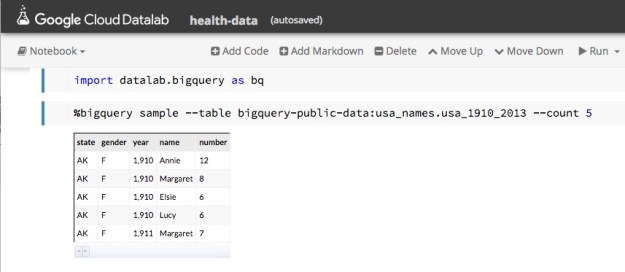
Figure 2. Sampling the names data.
This page gives us enough information about the schema that we can now formulate a query.
In modern America there is a movement to “post-gender” names. Typical examples cited on the web are “Dakota”, “Skyler” and “Tatum”. A very simple SQL query can be formulated to see how the gender breakdown for these names show up in the data. In Datalab, we can formulate the query as shown in Figure 3.
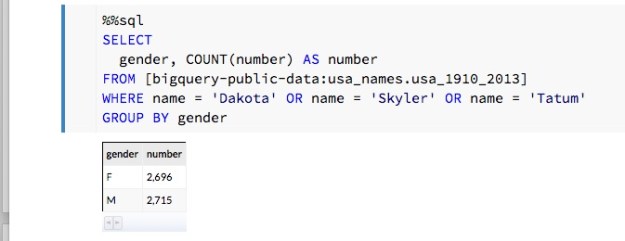
Figure 3. Breakdown by gender of three “post-gender” names.
As we can see, this is very nearly gender balanced. A closer inspection using each of the three names separately show that “Skyler” tends to be ‘F’ and “Tatum” tends to ‘M’. On the other hand, “Dakota” does seem to be truly post-gender with 1052 ‘F’ and 1200 ‘M’ occurrences.
We can also consider the name “Billy” which, in the US, is almost gender neutral. (Billy Mitchel was a famous World Work I general and also a contemporary Jazz musician. Both male. And Billy Tipton and Billy Halliday were female musicians though Billy Halliday was actually named Billie and Billy Tipton lived her life as a man, so perhaps they don’t count. We can ask how often Billy was used as a name associated with gender ‘F’ in the database? It turns out it is most common in the southern US. We can then group these by state and create a count and show the top five. The SQL command is easily inserted into the Datalab note book as shown in Figure 4.
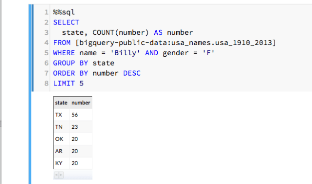
Figure 4. Search for Billy with gender ‘F’ and count and rank by state of birth.
Rubella in Washington and Indiana
A more interesting data collection is Center for Disease Control and Prevention dataset concerning diseases reported by state and city over a long period. An interesting case is Rubella, which is virus also known as the “German measles”. Through our vaccination programs it has been eliminated in the U.S. except for those people who catch it in other countries where it still exists. But in the 1960s it was a major problem with an estimated 12 million cases in the US and a significant number of newborn deaths and birth defects. The vaccine was introduced in 1969 and by 1975 the disease was almost gone. The SQL script shown below is a slight modified version of one from the Google Bigquery example. It has been modified to look for occurrences of Rubella in two states, Washington and Indiana, over the years 1970 and 1971.
%%sql --module rubella
SELECT
  *
FROM (
  SELECT
    *, MIN(z___rank) OVER (PARTITION BY cdc_reports_epi_week) AS z___min_rank
  FROM (
    SELECT
      *, RANK() OVER (PARTITION BY cdc_reports_state ORDER BY cdc_reports_epi_week ) AS z___rank
    FROM (
      SELECT
        cdc_reports.epi_week AS cdc_reports_epi_week,
        cdc_reports.state AS cdc_reports_state,
        COALESCE(CAST(SUM((FLOAT(cdc_reports.cases))) AS FLOAT),0)
         AS cdc_reports_total_cases
      FROM
        [lookerdata:cdc.project_tycho_reports] AS cdc_reports
      WHERE
        (cdc_reports.disease = 'RUBELLA')
        AND (FLOOR(cdc_reports.epi_week/100) = 1970
          OR FLOOR(cdc_reports.epi_week/100) = 1971)
        AND (cdc_reports.state = 'IN'
          OR cdc_reports.state = 'WA')
      GROUP EACH BY
        1, 2) ww ) aa ) xx
WHERE
  z___min_rank <= 500
LIMIT
  30000
We can now invoke this query as part of a python statement so we can capture its result as a pandas data frame and pull apart the time stamp fields and data values.
rubel = bq.Query(rubella).to_dataframe()
rubelIN = rubel[rubel['cdc_reports_state']=='IN']
                 .sort_values(by=['cdc_reports_epi_week'])
rubelWA = rubel[rubel['cdc_reports_state']=='WA']
                 .sort_values(by=['cdc_reports_epi_week'])
epiweekIN = rubelIN['cdc_reports_epi_week']
epiweekWA = rubelWA['cdc_reports_epi_week']
rubelINval = rubelIN['cdc_reports_total_cases']
rubelWAval = rubelWA['cdc_reports_total_cases']
At this point a small adjustment must be made to the time stamps. The CDC reports times in epidemic weeks and there are 52 weeks in a year. So the time stamps for the first week of 1970 is 197000 and the time stamp for the last week is 197051. The next week is 197100. To make these into timestamps that appear contiguous we need to make a small “time compression” as follows.
realweekI = np.empty([len(epiweekIN)])
realweekI[:] = epiweekIN[:]-197000
realweekI[51:] = realweekI[51:]-48
Doing the same thing with epiweekWA we now have the basis of something we can graph. Figure 5 shows the progress of rubella in Washington and Indiana over two years. Washington is the red line and Indiana is blue. Note that the outbreaks occur about the same time in both states and that by late 1971 the disease is nearly gone.
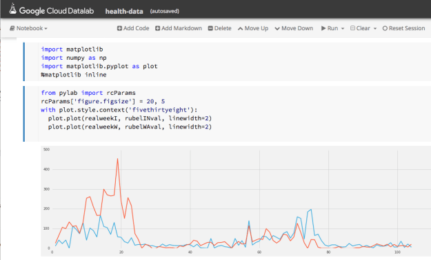
Figure 5. Progress of Rubella in Washington (red) and Indiana (blue) from 1970 through 1971.
Continuing the plot over 1972 and 1973 show there are flare-ups of the disease each year but their maximum size is diminishes rapidly.
(Datalab has some very nice plotting functions, but we could not figure out how to do a double plot, so we used the mathplot library with the “fivethirtheight” format.)
A Look at the Weather
From the national oceanographic and atmospheric administration we have the global summary of the day’s (GSOD) weather from the from 9000 weather stations between 1929 and 2016. While not all of these stations were operating during that entire period, there is still a wealth of weather data here. To illustrate it, we can use another variation on one of Google’s examples. Let’s find the hottest spots in the state of Washington for 2015. This was a particularly warm year that brought unusual droughts and fires to the state. The following query will list the hottest spots in the state for the year.
%%sql
SELECT
  max, (max-32)*5/9 celsius, mo, da, state, stn, name
FROM (
  SELECT
    max, mo, da, state, stn, name
  FROM
    [bigquery-public-data:noaa_gsod.gsod2015] a
  JOIN
    [bigquery-public-data:noaa_gsod.stations] b
  ON
    a.stn=b.usaf
    AND a.wban=b.wban
  WHERE
    state="WA"
    AND max
The data set ‘gsod2015’ is the table of data for the year 2015. To get a list that also shows the name of the station we need to do a join with the ‘station’ table over the corresponding station identifiers. We order the results descending from the warmest recordings. The resulting table is shown in Figure 6 for the top 10.
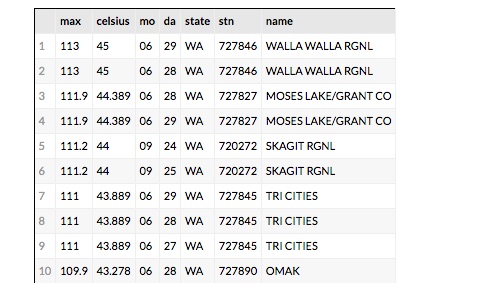
Figure 6. The top 10 hottest spots in Washington State for 2015
The results are what we would expect. Walla Walla, Moses Lake and Tri Cities are in the eastern part of the state and summer was very hot there in 2015. But Skagit RGNL is in the Skagit Valley near Puget Sound. Why is it 111 degrees F there in September? If it is hot there what was the weather like in the nearby locations? To find out which stations were nearby we can look at the stations on a map. The query is simple but it took some trial and error.
%%sql --module stationsx
DEFINE QUERY locations
  SELECT FLOAT(lat/1000.0) AS lat, FLOAT(lon/1000.0) as lon, name
  FROM [bigquery-public-data:noaa_gsod.stations]
  WHERE state="WA" AND name != "SPOKANE NEXRAD"
It seems that the latitude and longitude for the Spokane NEXRAD station are incorrect and resolve to some point in Mongolia. By removing it we get a good picture of the nearby stations as shown in Figure 7.
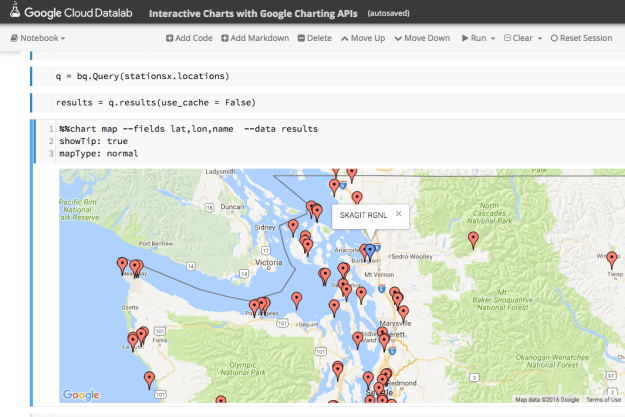
Figure 7. Location of weather stations in western Washington using the Bigquery chart map function.
This is an interactive map, so we can get the names of the nearby stations. There is one only a few miles away called PADILLA BAY RESERVE and the next closest is BELLINGHAM INTL. We can now compare the weather for 2015 at these three locations.
To get the weather for each of these we need the station ID. We can do that with a simple query.
%%sql
SELECT
  usaf, name
FROM [bigquery-public-data:noaa_gsod.stations]
WHERE
    name="BELLINGHAM INTL" OR name="PADILLA BAY RESERVE" OR name = "SKAGIT RGNL"
Once we have our three station IDs we can use the follow to build a parameterized Bigquery expression.
qry = "SELECT max AS temperature, \
       TIMESTAMP(STRING(year) + '-' + STRING(mo) + \
       '-' + STRING(da)) AS timestamp \
FROM [bigquery-public-data:noaa_gsod.gsod2015] \
WHERE stn = '%s' and max /< 500 \
ORDER BY year DESC, mo DESC, da DESC"

stationlist = ['720272','727930', '727976']

dflist = [bq.Query(qry % station).to_dataframe() for station in stationlist]
We can now render an image of the weather for our three stations as shown in Figure 8.
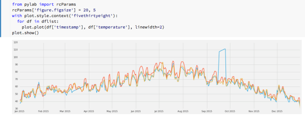
Figure 8. Max daily temperatures for Skagit (blue), Padilla Bay (red) and Bellingham (yellow)
We can clearly see the anomaly for Skagit in September and it is also easy to spot another problem in March where the instruments seemed to be not recording. Other than that there is close alignment of the readings.
Conclusions
There are many features of Datalab that we have not demonstrated here. The documentation gives an example of using Datalab with Tensorflow and the charting capabilities are more extensive than demonstrated here. (The Google maps example here was not reproducible in any other notebook beyond the demo in the samples which we modified to run the code here.) It is also easy to upload your own data to the warehouse and analyze it with Datalab.
Using Datalab is almost addictive. For every one of the data collections we demonstrated here there were many more questions we wanted to explore. For example, where and when did the name “Dakota” start being used and how did its use spread? Did the occurrence of Rubella outbreaks correspond to specific weather events? Can we automate the process of detecting non-functioning weather instruments over the years where records exist? These are all relatively standard data mining tasks, but the combination of Bigquery and IPython in the notebook format makes it fun.
It should be noted that Datalab is certainly not the first use of the IPython notebook as a front-end to cloud hosted analysis tools. The IPython notebook has been used frequently with Spark as we have previously described. Those interested in an excellent overview of data science using Python should look at “Python Data Science Handbook” by Jake VanderPlas which makes extensive use of IPython notebooks. There are a variety of articles about using Jupyter on AWS and Azure for data analytics. A good one is by Cathy Ye about deep learning using Jupyter in the cloud where she gives detailed instruction for how to install Jupyter on AWS and deploy Caffe there.
.

