Category Archives: deep neural nets

Revisiting Autoencoders

Abstract

We wrote about generative neural networks in two previous blog posts where we promised to return to the topic in a future update. This is it. This article is a review of some of more advances in autoencoders over the last 10 years. We present examples of denoising autoencoders, variational and three different adversarial neural networks. The presentation is not theoretical, and it uses examples via Jupyter notebooks that can be run on a standard laptop.

Introduction

Autoencoders are a class of deep neural networks that can learn efficient representations of large data collections. The representation is required to be robust enough to regenerate a good approximation of the original data. This can be useful for removing nose from the data when the noise is not an intrinsic property of the underlying data. These autoencoder often, but not always, work by projecting the data into a lower dimensional space (much like what a principal component analysis achieves). We will look at an example of a “denoising autoencoder” below where the underlying signal is identified through a series of convolutional filters.

A difference class of autoencoders are called Generative Autoencoders that have the property that they can create a mathematical machine that can reproduce the probability distribution of the essential features of a data collection. In other words, a trained generative autoencoder can create new instances of ‘fake’ data that has the same statistical properties as the training data. Having a new data source, albeit and artificial one, can be very useful in many studies where it is difficult to find additional examples that fit a given profile. This ideas is being used in research in particle physics to improve the search for signals in data and in astronomy where generative methods can create galaxy models for dark energy experiments.

A Denoising Autoencoder.

Detecting signals in noisy channels is a very old problem. In the following paragraphs we consider the problem of identifying cosmic ray signals in radio astronomy. This work is based on “Classification and Recovery of Radio Signals from Cosmic Ray Induced Air Showers with Deep Learning”, M. Erdmann, F. Schlüter and R. Šmída 1901.04079.pdf (arxiv.org) and Denoising-autoencoder/Denoising Autoencoder MNIST.ipynb at master · RAMIRO-GM/Denoising-autoencoder · GitHub. We will illustrate a simple autoencoder that pulls the signals from the noise with reasonable accuracy.

For fun, we use three different data sets. One is a simulation of cosmic-ray-induced air showers that are measured by radio antennas as described in the excellent book “Deep Learning for Physics Research” by Erdmann, Glombitza, Kasieczka and Klemradt. The data consists of two components: one is a trace of the radio signal and the second is a trace of the simulated cosmic ray signal. A sample is illustrated in Figure 1a below with the cosmic ray signal in red and the background noise in blue. We will also use a second data set that consists of the same cosmic ray signals and uniformly distributed background noise as shown in Figure 1b. We will also look at a third data set consisting of the cosmic ray signals and a simple sine wave noise in the background Figure 1c. As you might expect, and we will illustrate, this third data set is very easy to clean.

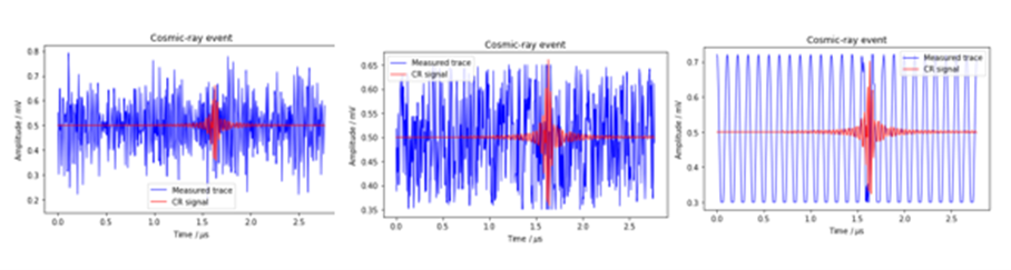
Figure 1a, original data Figure 1b, uniform data Figure 1c, cosine data

To eliminate the nose and recover the signal we will train an autoencoder based on a classic autoencoder design with an encoder network that takes as input the full signal (signal + noise) and a decoder network that produces the cleaned version of the signal (Figure 2). The projection space in which the encoder network sends in input is usually much smaller than the input domain, but that is not the case here.

Figure 2. Denoising Autoencoder architecture.

In the network here the input signals are samples in [0, 1]⁵⁰⁰. The projection of each input consists of 16 vectors of length 31 that are derived from a sequence of convolutions and 2×2 pooling steps. In other words, we have gone from a space of dimension 500 to 496. Which is not a very big compression. The details of the network are shown in Figure 3.

The one dimensional convolutions act like frequency filters which seem to leave the high frequency cosmic ray signal more visible. To see the result, we have in figure 4 the output of the network for three sample test examples for the original data. As can be seen the first is a reasonable reconstruction of the signal, the second is in the right location but the reconstruction is weak, and the third is completely wrong.

Figure 3. The network details of the denoising autoencoder.

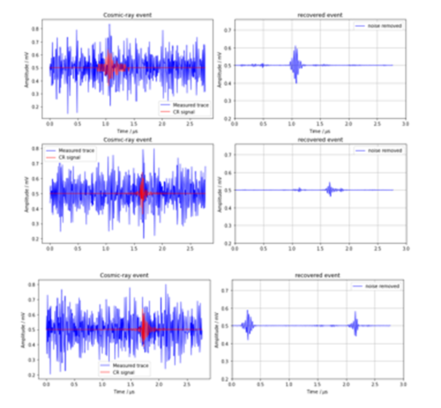
Figure 4. Three examples from the test set for the denoiser using the original data

The two other synthetic data sets (uniformly distributed random nose and noise create from a cosine function) are much more “accurate”.

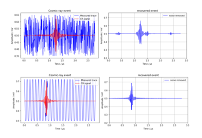
Figure 5. Samples from the random noise case (top) and the cosine noise case (bottom)

We can use the following naive method to assess accuracy. We simply track the location of the reconstructed signal. If the maximum value of the recovered signal is within 2% of the maximum value of the true signal, we call that a “true reconstruction”. Based on this very informal metric we see that the accuracy for the test set for the original data is 69%. It is 95% for the uniform data case and 98% for the easy cosine data case.

Another way to see this result is to compare the response in the frequency domain, by applying an FFT to the input and output signals we see the results in Figure 6.

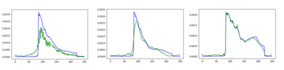
Figure 6a, original data Figure 6b, uniform data Figure 6c, cosine data

The blue line is the frequency spectrum of the true signal, and the green line is the recovered signal. As can be seen, the general profiles are all reasonable with the cosine data being extremely accurate.

Generative Autoencoders.

Experimental data drives scientific discovery. Data is used to test theoretical models. It is also used to initialize large-scale scientific simulations. However, we may not always have enough data at hand to do the job. Autoencoders are increasingly being used in science to generate data that fits the probabilistic density profile of known samples or real data. For example, in a recent paper, Henkes and Wessels use generative adversarial networks (discussed below) to generate 3-D microstructures for studies of continuum micromechanics. Another application is to use generative neural networks to generate test cases to help tune new instruments that are designed to capture rare events.

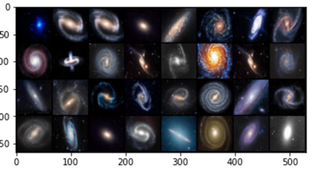
In the experiments for the remainder of this post we use a very small collection of images of Galaxies so that all of this work can be done on a laptop. Figure 7 below shows a sample. The images are 128 by 128 pixels with three color channels.

Figure7. Samples from the Galaxy image collection

Variational Autoencoders

A variational autoencoder is a neural network that uses an encoder network to reduce data samples to a lower dimensional subspace. A decoder network takes samples from this hypothetical latent space and uses it to regenerate the samples. The decoder becomes a means to map a uniform distribution on this latent space into the probability distribution of our samples. In our case, the encoder has a linear map from the 49152 element input down to a vector of length 500. This is then mapped by a 500 by 50 linear transforms down to two vectors of length 50. The decoder does a renormalization step to produce a single vector of length 50 representing our latent space vector. This is expanded by two linear transformations are a relu map back to length 49152. After a sigmoid transformation we have the decoded image. Figure 8 illustrates the basic architecture.

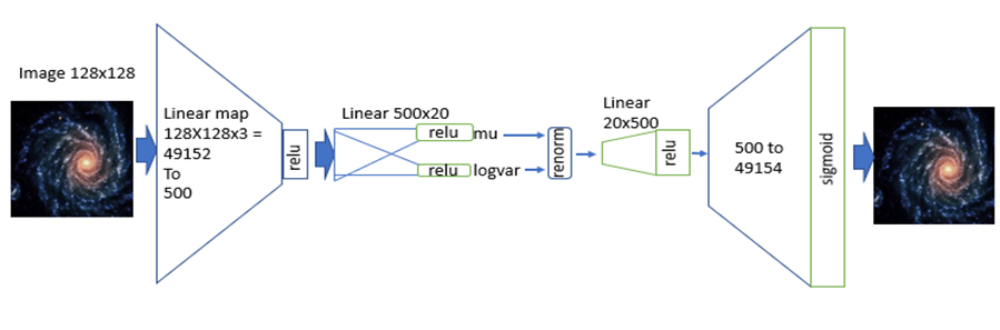
Figure 8. The variational autoencoder.

Without going into the mathematics of how this works (for details see our previous post or the “Deep Learning for Physics Research” book or many on-line sources), the network is designed so that the encoder network generates mean (mu) and standard deviation (logvar) of the projection of the training samples in the small latent space such that the decoder network will recreate the input. The training works by computing the loss as a combination of two terms, the mean squared error of the difference between the regenerated image and the input image and Kullback-Leibler divergence between the uniform distribution and the distribution generated by the encoder.

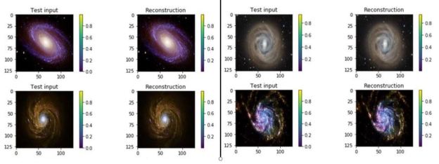
The Pytorch code is available as a the notebook in github. The same github directory contains the zipped datafile). Figure 9 illustrates the results of the encode/decode on 8 samples from the data set.

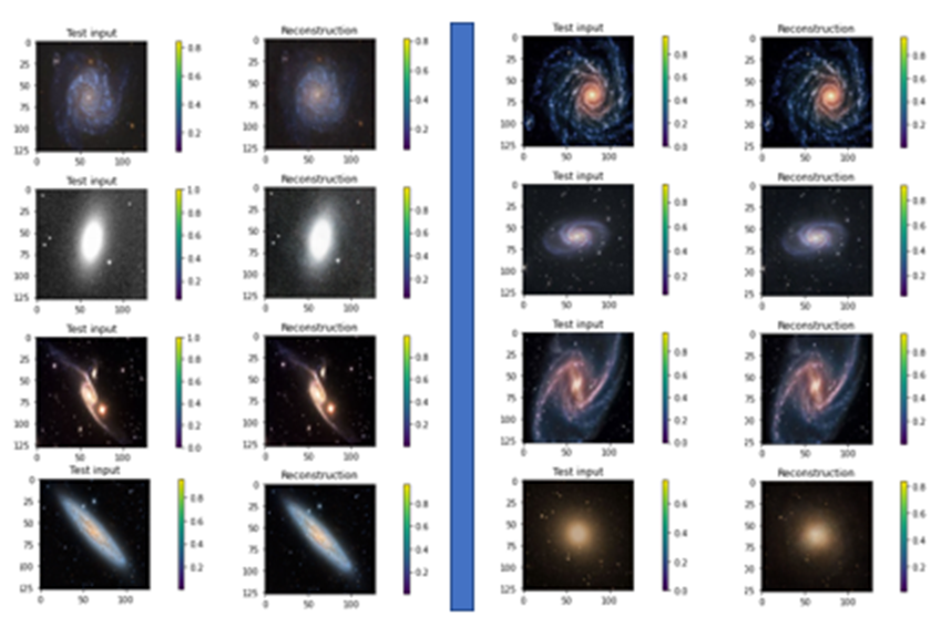
Figure 9. Samples of galaxy images from the training set and their reconstructions from the VAR.

An interesting experiment is to see how the robust the decoder is to changes in the selection of the latent variable input. Figure 10 illustrates the response of the decoder when we follow a path in the latent space from one instance from the training set to another very similar image.

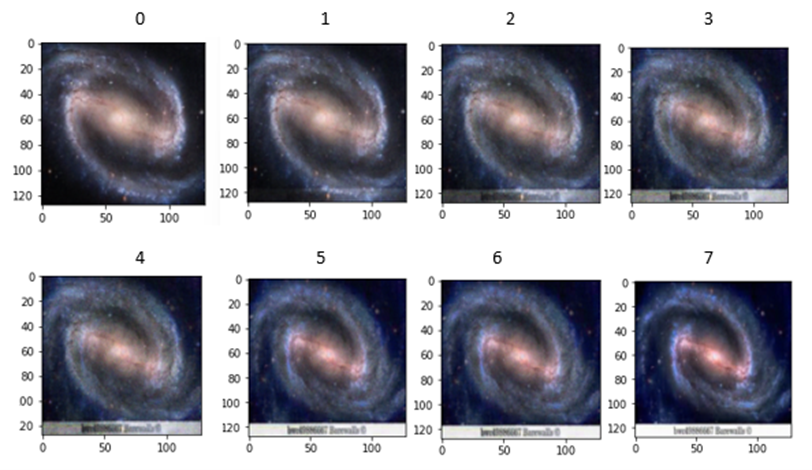
Figure 10. image 0 and image 7 are samples from the training set. Images 1 through 6 are generated from points along the path between the latent variable for 0 and for 7.

Another interesting application was recently published. In the paper “Detection of Anomalous Grapevine Berries Using Variational Autoencoders” Miranda et.al. show how a VAR can be used to examine arial photos of vineyards to spot areas of possible diseased grapes.

Generative Adversarial Networks (GANs)

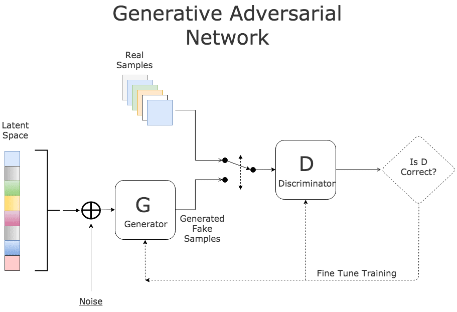
Generative Adversarial networks were introduced by Goodfellow et, al (arXiv:1406.2661) as a way to build neural networks that can generate very good examples that match the properties of a collection of objects.

As mentioned above, artificial examples generated by autoencoder can be used as starting points for solving complex simulations. In the case of astronomy, cosmological simulation is used to test our models of the universe. In “Creating Virtual Universes Using Generative Adversarial Networks” (arXiv:1706.02390v2 [astro-ph.IM] 17 Aug 2018) Mustafa Mustafa, et. al. demonstrates how a slightly-modified standard GAN can be used generate synthetic images of weak lensing convergence maps derived from N-body cosmological simulations. In the remainder of this tutorial, we look at GANs.

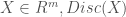
Given a collection r of objects in R^m, a simple way to think about a generative model is as a mathematical device that transforms samples from a multivariant normal distribution N^k(0,1) into R^m so that they look like they come from the actual distribution Pr. for our collection r. Think of it as a function

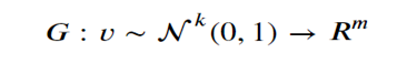
Which maps the normal distribution into a distribution Pg over R^m.

In addition, assume we have a discriminator function

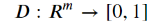
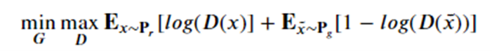
With the property that D(x) is the probability that x is in our collection r. Our goal is to train G so that Pg matches Pr. Our discriminator is trained to reject images generated by the generator while recognizing all the elements of Pr_.The generator is trained to fool the discriminator, so we have a game defined by minimax objective:

We have put a simple basic GAN from our previous post. Running it for many epochs can occasionally get some reasonable results as shown if Figure 11. While this looks good, it is not. Notice that it generated examples of only 3 of our samples. This repeating of an image for different latent vectors is an example of a phenomenon called modal collapse.

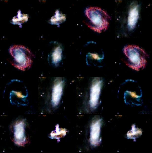
Figure 11. The lack of variety in the images is called model collapse.

acGAN

There are several variations on GANs that avoid many of these problems. One is called an acGAN for auxiliary classifier Gan developed by Augustus Odena, Christopher Olah and Jonathon Shlens. For an acGan we assume that we have a class label for each image. In our case the data has three categories: barred spiral (class 0), elliptical (class 1) and spiral (class 2). The discriminator is modified so that it not only returns the probability that the image is real, it also returns a guess at the class. The generator takes an extra parameter to encourage it to generate an image of the class. Let d-1 = the number of classes then we have the functions

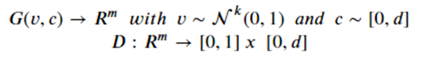
The discriminator is now trained to minimize the error in recognition but also the error in class recognition. The best way to understand the details is to look at the code. For this and the following examples we have notebooks that are slight modifications to the excellent work from the public Github site of Chen Kai Xu from Chen Kai Xu Tsukuba University. This notebook is here. Figure 12 below shows the result of asking the generator to create galaxies of a given class. The G(z,0) generates good barred spirals, G(z,1) are excellent elliptical galaxies and G(z,2) are spirals.

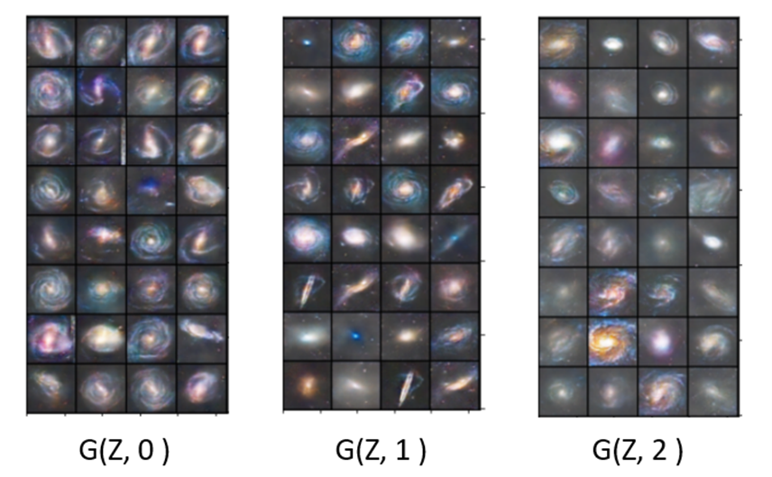
Figure 12. Results from asgan-new. Generator G with random noise vector Z and class parameter for barred spiral = 0, elliptical = 1 and spiral = 2.

Wasserstein GAN with Gradient Penalty

The problem with modal collapse and convergence failure was, as stated above, commonly observed. The Wasserstein GAN introduced by Martin Arjovsky , Soumith Chintala , and L´eon Bottou, directly addressed this problem. Later Ishaan Gulrajani, Faruk Ahmed, Martin Arjovsky, Vincent Dumoulin and Aaron Courville introduced a modification called a Gradient penalty which further improved the stability of the GAN convergence. To accomplish this they added an additional loss term to the total loss for training the discriminator as follows:

Setting the parameter lambda to 10.0 this was seen as an effective value for reducing to occurrence of mode collapse. The gradient penalty value is computed using samples from straight lines connecting samples from Pr and Pg. Figure 13 shows the result of a 32 random data vectors for the generator and the variety of responses reflect the full spectrum of the dataset.

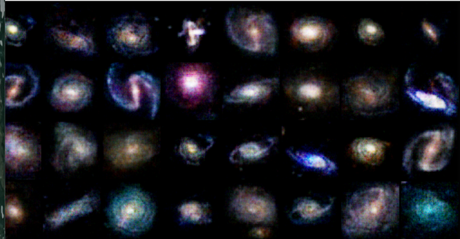
Figure 13. Results from Wasserstein with gradient penalty.

The notebook for wgan-gp is here.

Wasserstein Divergence for GANs

Jiqing Wu , Zhiwu Huang, Janine Thoma , Dinesh Acharya , and Luc Van Gool introduced a variation on WGAN-gp called WGAN-div that addresses several technical constraints of WGAN-gp having to do with Lipschitz continuity not discussed here (see the paper). They propose a better loss function for training the discriminator:

By experimental analysis the determine the best choice for the k and p hyperparameters are 2 and 6.

Figure 14 below illustrates the results after 5000 epochs of training. The notebook is here.

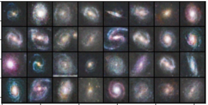
Figure 14. Results from WG-div experiments.

Once again, this seems to have eliminated the modal collapse problem.

Conclusion

This blog was written to do a better job illustrating autoencoder neural networks than our original articles. We illustrated a denoising autoencoder, a variational autoencoder and three generative adversarial networks. Of course, this is not the end of the innovation that has taken place in this area. A good example of recent work is the progress made on Masked Autoencoders. Kaiming He et. al. published Masked Autoencoders Are Scalable Vision Learners in December 2021. The idea is very simple and closely related to the underlying concepts used in Transformers for natural language processing like BERT or even GPT3. Masking simply removes patches of the data and trains the network to “fill in the blanks”. The same idea has been now applied to audio signal reconstruction. These new techniques show promise to generate more semantic richness to the results than previous methods.

eScience 2050: A Look Back

Abstract— This was originally written as an invited “vision” presentation for the eScience 2019 conference, but I decided to present something more focused for that event. Never wanting to let words go to waste I decided to put a revised version here. It was written as a look back at the period of eScience from 2019 to 2050. Of course, as it is being published in 2019, it is clearly a work of science fiction, but it is based on technology trends that seem relatively clear. Specifically, I consider the impact of four themes on eScience: the explosion of AI as an eScience enabler, quantum computing as a service in the cloud, DNA data storage in the cloud, and neuromorphic computing.

I. Introduction

Predictions of the future are often so colored by the present that they miss the boat entirely. The future, in these visions, tends to look like today but a bit nicer. Looking at images of the future from the 1950s we see pictures of personal helicopters (Figure 1) that clearly missed the mark. But in some cases, the ideas are not so far off, as in the case of the woman ordering shirts “online” as in Figure 2.

Fig 1. Future personal transportation. Mechanics Illustrated, Jan 1951

Fig 2. Shopping “online” vision.

To look at the evolution of eScience in the period from 2019 to 2050, it can help to look at the state of the art in computing in 1960 and ask how much of todays technology can we see emerging there. My first computer program was written when I was in high school. It was a Fortran version of “hello world” that consited of one line of Fortran per punched card as shown in Figure 3 and the entire program consisted of a deck of 12 cards .

Fig 3. The Fortran statement CALL RCLASS(AAA,21,NNC, PX3,PX4)

If asked to predict the future then, I might have said that software and data in the years ahead would be stored on a punched paper tape over ten miles long.

Fifty years ago, the high points of computing looked like:

The programming language FORTRAN IV was created in 1961.
IBM introduced its System/360. A monster machine.
Gordon Moore makes an observation about scale in 1965 (that became Moore’s law).
IBM created the first floppy disk in 1967.
The SABRE database system that was used by IBM to help American Airlines manage its reservations data.
In 1970 Edgar Codd came up with Relation Database Idea. It was not implemented until 1974.
The Internet: a UCLA student, tries to send “login,” the first message over ARPANET, at 10:30 P.M. on October 29, 1969. (The system transmitted “l” and then “o” …. and then crashed.)

What we can extrapolate from this is that mainframe IBM computers will continue to dominate, databases are going to emerge as a powerful tool and there will be a future for computer-to-computer networking, but PCs and web search were not remotely visible on the horizon. The profound implication of Moore’s law would not be evident until the first microprocessors appear in 1979 and the personal computer revolution of the 1980s followed. Those same microprocessors led to the idea that dozens of them could be packaged into a “parallel computer”. This resulted in a period of intense research in universities and startups to build scalable parallel systems. While the first massively parallel computer was the Illiac IV which was deployed at NASA Ames in 1974, it was the work on clusters of microprocessors in the 1980s [1] that led to the supercomputers of 2019. Looking at computing in 1970, few would have guessed this profound transition in computing from mainframes like the System/360 to the massively parallel systems of 2019.

II. eScience from 2019 Forward

A. The Emergence and Evolution of the Cloud

The World Wide Web appeared in 1991 and the first search engines appeared in the mid 90s. As these systems evolved, so did the need to store large segments of the web on vast server farms. Ecommerce also drove the need for large data centers. These data centers quickly evolved to offering data storage and virtual machines as a service to external users. These clouds, as they became known, were designed to serve thousands to millions of concurrent clients in interactive sessions.

For eScience, clouds provided an important alternative to traditional batch-oriented supercomputers by supporting interactive, data exploration and collaboration at scale. The cloud data centers evolved in several important way. Tools like Google’s Kubernetes was widely deployed to support computation in the form of swarms of microservices built from software containers. Deploying Kubernetes still required allocating resources and configuring systems and microservices are continuously running processes. Serverless computing is a newer cloud capability that avoids the need to configure VMs to support long running processes when they are not needed.

Serverless computing is defined in terms of stateless functions that respond to events such as signals from remote instruments or changes in the state of a data archive. For examples, an eScience workflow can be automatically triggered when instrument data arrives in the data storage archive. The analysis in the workflow can trigger other serverless function to complete additional tasks.

The Cloud if 2019 is defined in terms of services and not raw hardware and data storage. These services include

Streaming data analytics tools that allow the users to monitor hundreds of live streams from remote instruments. Edge computing services evolved as a mechanism to off-load some of the analytics to small devices that interposed between the instruments and the cloud.
Planet scale databases allow a user to store and search data collections that are automatically replicated across multiple continents with guaranteed consistency.
Services to support applications of machine learning became widely available across all the commercial public clouds. These services include speech recognition and generation, automatic language translation, computer vision tasks such as image recognition and automatic captioning.

The architecture of the cloud data centers continued to evolve toward ideas common in modern supercomputers. The first major change was the introduction of software defined networking throughout the data centers. Amazon began introducing GPU accelerators in 2012. This was followed by Google’s introduction of TPU chips to support the computational needs of deep learning algorithms coded in the Tensorflow system. The TPU (figure 4) is a device designed to accelerate matrix multiplication. It is based on systolic computation ideas of the 1980s and has been applied primarily to Google machine learning projects.

Fig 4. Google TPU v3 architecture. See N. Jouppi, C. Young, N. Patil, D. Patterson [2, 3].

The most radical evolutionary step has been taken by Microsoft in the Azure cloud. Project Brainwave represents an introduction of a mesh connected layer of FPGA devices that span the entire data center (figure 5). These devices can be programed to cooperate on parallel execution of lage computational task including serving deep learning models.Fig 5. Microsoft FPGA based Project Brainwave [4, 5]

A. Major Themes Going Forward from 2019

The following pages will describe the four major themes that are going to dominate the ten years forward from 2019. They are

The explosion of AI as an eScience enabler.
Quantum computing as a service in the cloud.
DNA data storage in the cloud.
Neuromorphic computing

III. AI and eScience

Machine Learning went through a revolution in the years from 2008 to 2019 due to the intensive work at universities and in companies. The cloud providers including Google, Microsoft and others were driven by the need improve their search engines. Along the way they had amassed vast stores of text and images. Using this data and the new deep learning technologies they were able to build very powerful language translations systems and image recognition and captioning services that were mentioned above. By 2017, applications to eScience were beginning to emerge.

A. Generative Neural Networks and Scientific Discovery

One of the more fascinating developments that arose from the deep learning research was the rise of a special class of neural networks called generative models. The important property of these networks is that if you train them with a sufficiently, large and coherent collection of data samples, the network can be used to generate similar samples. These are most often seen in public as pernicious tools to create fake images and videos of important people saying things they never said.

What these networks are doing is creating a statistical distribution of data that, when sampled, produces data that has properties that match nicely with the input data. When a scientist creates a simulation based on assumed parameters of nature, the simulations is evaluated against the statistical properties of the experimental observations. Generative models can be used to validate the simulation output in case the data is sparse. One of the most commonly used generative model is the Generative Adversarial Network (GAN) in which to networks are pitted against each other. As shown in Figure 6, a discriminator is trained to recognize the data that is from the real data set and a generator is designed to fool the discriminator. When converged the generator mimics the data distribution of the real data. There are several interesting examples of how generative models have been used in science. We list several in [6], but two that stand out are an application in astronomy and one in drug design.

Fig 6. Generative Adversarial Network (GAN) from this site.

M. Mustafa, and colleagues demonstrate how a slightly-modified standard Generative Adversarial Network (GAN) can be used generate synthetic images of weak lensing convergence maps derived from N-body cosmological simulations [7]. The results illustrate how the generated images match their validation tests, but what is more important, the resulting images also pass a variety of statistical tests ranging from tests of the distribution of intensities to power spectrum analysis.

However, generative methods do not, by themselves, help with the problem of inferring the posterior distribution of the inputs to scientific simulations conditioned on the observed results, but there is value of in creating ‘life-like’ samples. F. Carminati, G. Khattak, S. Vallecorsa make the argument that designing and testing the next generation of sensors requires test data that is too expensive to compute with simulation . A well-tuned GAN can generate the test cases that fit the right statistical model at the rate needed for deployment [8].

In the area of drug design, Shahar Harel and Kira Radinsky have used a generative model to suggest chemical compounds that may be used as candidates for study [9]. They start with a prototype compound known to have some desirable properties. This is expressed as sequence and fed to a layer of a convolutional network that allow local structures to emerge as shorter vectors that are concatenated. A final all-to-all layer is used to generate sequence of mean and variance vectors for the prototype. his is fed to a “diversity layer” which add randomness as shown in Figure 7.

Fig 7. Shahar Harel and Kira Radinsky multi-layer generative netowork for drug design.

The decoder is an LSTM-based recurrent network which generates the new molecule. The results they report are impressive. In a one series of experiments they took as prototypes compounds from drugs that were discovered years ago, and they were able to generate more modern variations that are known to be more powerful and effective. No known drugs were used in the training.

B. Probabilistic Programming and Bayesian Inference

For very large experiments such as those conducted in the Large Hadron Collider, the scientists are interested in testing their models of the universe based the record of particle collisions that were generated. It is often the case that the scientists have a detailed simulation of the experimental system based on the current theoretical models of physics that are involved. These models are driven by setting parameters that correspond to assumptions about nature. When they run the experiment, they see new behaviors in the data, such as new particles emerging from collisions, and they would like to see which parameters when fed to the simulation can produce the output that corresponds to the experimental results. In other words, the simulation is a function taking parameters x to outputs y and the interesting question is given the outputs what the corresponding values for x. This is an inverse problem that is notoriously difficult to solve for large scientific problems. In terms of Bayesian statistics, they are interested in the posterior distribution P(x | y) where y is the experimental statistics.

In 2018 and later researchers began to study programming languages designed to express and solve problems like these. Pyro [10], Tensorflow Probability [11], and the Julia-based Gen [12] are a few of the Probabilistic Programing Languages (PPLs) introduced in 2019. One of the ideas in these languages is to build statistical models of behavior where program variables represent probability distributions and then, by looking at traces of the random choices associated with these variables during execution, one can make inferences about the random behaviors that influence outcomes.

These languages have been put in use in industries such as finance, their role in eScience is now becoming apparent. A. Güneş Baydin, et al. showed that PPLs can be used in very large Bayesian analysis of data from an LHC use case. Their approach allows a PPL too couple directly to existing scientific simulators through a cross-platform probabilistic execution protocol [13].

Probabilistic programming with PPLs will go on to become a standard tool used by eScientists.

C. AI-based Research Assistant

2018 was the year of the smart on-line bot and smart speaker. These were cloud based services that used natural language interfaces for both input and output. The smart speakers, equipped with microphones listen for trigger phrases like “Hello Siri” or “hello Google” or “Alexa” and recorded a query in English, extracted the intent and replied within a second. They could deliver weather reports, do web searches, keep your shopping list and keep track of your online shopping.

The impact of this bot technology will hit eScience when the AI software improves to the point that every scientist, graduate student and corporate executive had a person cloud-based research assistant. Raj Reddy calls these Cognition Amplifiers and Guardian Angels. Resembling a smart speaker or desktop/phone app, the research assistant is responsible for the following tasks:

Cataloging research data, papers and articles associated with its owner’s projects. The assistant will monitor the research literature looking for papers exploring the same concepts seen in the owner’s work.
Coordinate meetings among collaborators and establish coordination among other research assistants.
Automatically sifting through other data from collaborators and open source archives that may be of potential use in current projects.
Understanding the mathematical analysis in the notes generated by the scientist and using that understanding to check proofs and automatically propose simulators and experiment designs capable of testing hypotheses implied by the research.

From the perspective of 2019 eScience, the claim that the Research Assistant of the future will be able to derive simulations and plan experiments may seem a bit “over the top”. However, progress on automatic code completion and generation was making great strides in 2019. Transformers [16] provide a second generation of sequence-to-sequence AI tools that outpaced the recurrent neural networks previously used. Advances in programming tools based on similar technology show that AI can be used to generate code completions for C# method calls based on deep semantic mining of online archives of use cases.

We built a toy demo of the Research Assistant in [14] that could take natural language (spoken or typed) input and find related research articles from Bing, Wikipedia and ArXiv (see Figure 6.)

Fig 6. Demo cloud-based “research assistant” [14]

This demo prototype research assistant was built by composing a few cloud tools as shown in Figure 7. A much more sophisticated version can be built using a modern chatbot tool like RASA, but that will not address everything that is needed to reach the final goal.

Fig 7. The toy research assistant demo is hosted an “elegant” cardboard container from Google’s voice kit running a python script on raspberry Pi. It invokes Googles speech to text, a text analysis service running on Algorithmia and uses Amazon’s Lex to generate voice. Depending on context, calls are made to Bing, Wikipedia or ArXiv.

While this demo was a toy, there has been serious work over the last few years to make progress on this topic. In 2018, Google introduced its Dataset Search service to provide easy data set discovery. The work of the Allen Institute for AI stands out [15]. Their Semantic Sanity project is a sophisticated research search engine that allows you to tell it basic topics that interest you and it will monitor ArXiv looking for important related contributions. Aristo is “an intelligent system that reads, learns, and reasons about science”. It can reason about diagrams, math and understand and answer elementary school science questions.

One important problem that must be solved is extracting non-trivial mathematical concepts from research papers and notes so that similar papers can be found. In addition to Semantic Sanity, there is some other early related work on this problem. For example, researchers are using unsupervised neural net to sift through PubChem and uses NLP techniques to identify potential components for materials synthesis [22].

IV. The Rise of Quantum in the Cloud

Long viewed as a subject of purely theoretical interest, quantum computing emerged in 2018 as a service in the cloud. By 2019, Rigetti, IBM, D-Wave and Alibaba had live quantum computing services available. Google and Microsoft followed soon after that. The approaches taken to building a quantum computer differed in many respects.

The basic unit of quantum computing is the qubit which obeys some important and non-intuitive laws of physics. Multiple qubits can be put into an “entangled” state in which an observation about one can effect the state of the others even when they are physically separated. One can apply various operators to qubits and pairs of qubits to form “logical” circuits and these circuits are the stuff of quantum algorithms. A fact of life about quantum states is that once you measure them, they are reduced to ordinary bits. However, the probability that a bit is reduced to a zero or a one is determined by the unmeasured quantum state of the system. A good quantum algorithm is one in which the quantum circuit produces outputs with a probability distribution that makes solving a specific problem very fast.

The first important quantum computations involved solving problems in quantum chemistry. In fact, this was the role that Richard Feynman had suggested for a quantum computer when he first came up with the idea in the 1980s. The other area of eScience that quantum computers excelled at was certain classes of optimization problems.

Early quantum computers are program by literally composing the quantum gates as illustrated in Figure 8.

Fig 8. A simple quantum circuit to create an entangled pair of two qubits and measure the result

Programming tools to build such circuits include IBM’s IBM-Q qiskit and Microsoft’s Q# language and compiler. The IBM hardware was based what they call “noisy intermediate-scale quantum computers (NISQ)”. As shown in Figure 9, the induvial qubits are non-linear oscillators. Tuned superconducting resonator channels are used for readout. Also, the qubits are tied together by additional superconducting channels

Fig 9 An early 5-qubit IBM-Q computational unit. Source: IBM-Q website.

One problem with early quantum systems is that the qubits are very susceptible to noise and degrade quickly. In other words, the error rate of quantum algorithms can be very high. The deeper the quantum circuit (the number of layers of “gates”), the more noise. A way around this is to add error-correcting redundancy into the circuit, but this means more qubits are required. Quantum volume refers to a measure of the number of qubits needed for the error-corrected circuit times the depth of the corrected circuit. Unfortunately, early quantum computers had very low bounds on achievable quantum volume.

Microsoft took a different approach to building qubits that are based on the topological property of woven threads. These are much more noise resistant and hence capable of building deeper circuits with less error correction.

IV. DNA-Based Storage

There are two problems with 2019 era storage technologies. First, it was not very stable. Data degrades and storage devices fail. Second, there was not enough storage capacity to capture the data that was being generated. 2.5 quintillion bytes of data was generated each day in 2018. Even if you cast out 99.9% of this as being of no long-term value, the remainder still leaves 2.5e+15 bytes per day. The amount of data stored in the cloud in 2018 was 1.0e+18 (an exabyte). In other words, the cloud only held 400 days’ worth of the important data. Obviously, another order or magnitude or more of the data needed to be discarded to allow the data centers time to expand to contain this growth. A new storage technology was needed.

DNA storage was first proposed in the 1960, but not much happened with the idea until 1988 when researchers from Harvard stored an image in the DNA of e.coli. By 2015 researchers at Columbia University published a method that allowed the storage of 215 petabytes (2.15e+17) of data per gram of DNA. And DNA is very stable over long periods of time. While this was promising, there was still a big problem. The encoding and decoding of the data were still an expensive manual process and it was not practical to have lab scientists running around in the back rooms of data centers managing wet processes.

In 2019, researchers at the University of Washington and Microsoft demonstrated an automated lab that could encode and decode data to DNA without human hands. The system works by converting the ones and zeros of digital data into the As, Ts, Cs and Gs that make up the building blocks of DNA. These encoded sequences are then fed into synthesizing systems. Their next breakthrough was to reduce the entire “lab” to a chip that uses microfluidics to route droplets of water around a grid to enact the needed chemistry steps. They also produced a sophisticated software stack called puddle that allow the scientist to program this with conventional high-level languages [20].

Other research has demonstrated ways in which DNA encoded data could be searched and structured in ways like relational databases. As the costs came down, this became the standard cloud storage technology.

VI. Neuromorphic Computing

It was long a dream of computer designers to build systems that mimicked the connectome of the biological brain. A major research initiative in Europe, the Human Brain Project, looked at the possibility of simulation a brain on traditional supercomputers. As that proved unrealistic, they turned to the study of special hardware devices that can simulate the behavior of neuron. Technology to build artificial neurons progressed in university and industry labs. The Stanford neurogrid can simulate six billion synapses. In 2017 Intel introduced the Loihi neuromorphic research test chip. The device is a many-core mesh of 128 neuromorphic cores and each of which contains 1,024 primitive spiking neural units. The neural units are current-based synapse leaky integrate-and-fire neurons [21].

In addition to the Loihi chip, Intel has released Pohoiki Beach, a system comprised of 64 Loihi chips and a substantial software stack to allow application development. Because overall power consumption is 100 times lower than GPU based neural networks, Intel’s application target is autonomous vehicles and robots. While full realization of true biological brain-like functionality may not be realized until the 2^nd half of the 21^st century, it is none the less an exciting step forward.

VII. Conclusions

EScientists in 2019 found themselves at an important inflection point in terms of the technology they could deploy in doing science. The cloud has evolved into a massive on-line, on-demand, heterogeneous supercomputer. It not only supports traditional digital simulation; it will also support hybrid quantum-digital computation. It will soon allow applications to interact with robotic sensor nets controlled by neuromorphic fabrics. Storage of research data will be limitless and backed up by DNA based archives.

One of the most remarkable features of computing in the 21^st century has been the evolution of software. Programming tools have evolved into very deep stacks that have used and exploited AI methods to enable scientific programmer to accomplish more with a few lines of Julia in a Juypter notebook than was remotely possible programming computers of 1980. New probabilistic programming languages that combine large scale simulation with deep neural networks show promise of making Bayesian inference an easy to use used tool in eScience.

The role of AI was not limited to the programming and execution of eScience experiments. Users of the AI research assistants in 2050 can look back at the “smart speakers” of 2019 and view them as laughably primitive as the users of the 2019 World Wide Web looked back at the 1970s era where computers were driven by programs written on decks of punched cards.

References

G. Fox, R. Williams, P. Massina, “Parallel Computing Works!”, Morgan Kauffman, 1994.
N. Jouppi, C. Young, N. Patil, D. Patterson, “A Domain-Specific Architecture for Deep Neural Networks”, Communications of the ACM, September 2018, Vol. 61 No. 9, Pages 50-59
https://cloud.google.com/tpu/docs/images/tpu-sys-arch3.png
Chung, et al. “Serving DNNs in Real Time at Datacenter Scale with Project Brainwave.” IEEE Micro 38 (2018): 8-20.
Fowers et al., “A Configurable Cloud-Scale DNN Processor for Real-Time AI,” 2018 ACM/IEEE 45th Annual International Symposium on Computer Architecture (ISCA), Los Angeles, CA, 2018, pp. 1-14
D. Gannon, “Science Applications of Generative Neural Networks”, https://esciencegroup.com/2018/10/11/science-applications-of-generative-neural-networks/, 2018
Mustafa, et. al. “Creating Virtual Universes Using Generative Adversarial Networks” (arXiv:1706.02390v2 [astro-ph.IM] 17 Aug 2018)
Carminati, G. Khattak, S. Vallecorsa, “3D convolutional GAN for fast Simulation”, https://www.ixpug.org/images/docs/IXPUG_Annual_ Spring_Conference_2018/11-VALLECORSA-Machine-learning.pdf
Harel and K. Radinsky, “Prototype-Based Compound Discovery using Deep Generative Models” http://kiraradinsky.com/files/acs-accelerating-prototype.pdf
Bingham, et al, “Pyro: Deep universal probabilistic programming.” Journal of Machine Learning Research (2018).
Tensorflow Probability, https://medium.com/tensorflow/an-introduction-to-probabilistic-programming-now-available-in-tensorflow-probability-6dcc003ca29e
Gen, https://www.infoq.com/news/2019/07/mit-gen-probabilistic-programs
Güneş Baydin, et al, “Etalumis: Bringing Probabilistic Programming to Scientific Simulators at Scale”, arXiv:1907.03382v1
Gannon, “Building a ‘ChatBot’ for Scientific Research”, https://esciencegroup.com/2018/08/09/building-a-chatbot-for-scientific-research
Allen Institute for AI, Semantic Sanity and Aristo, https://allenai.org/demos
Vaswani et al., “Attention Is All You Need”, arXiv:1706.03762v5
Chong, Hybrid Quantum-Classical Computing https://www.sigarch.org/hybrid-quantum-classical-computing/
Shaydulin, et al., “A Hybrid Approach for Solving Optimization Problems on Small Quantum Computers,” in Computer, vol. 52, no. 6, pp. 18-26, June 2019.
Takahashi, B. Nguyen, K. Strauss, L. Ceze, “Demonstration of End-to-End Automation of DNA Data Storage”, Nature Scientific Reports, vol. 9, no. 1, pp. 2045-2322, 2019
Wellsey, et al., “Puddle: A Dynamic, Error-Correcting, Full-Stack Microfluidics Platform”, ASPLOS’19 , April 13–17, 2019.
Intel Loihi Neurmorphic Chip. https://en.wikichip.org/wiki/intel/loihi
E. Kim, et al., “Materials Synthesis Insights from Scientific Literature via Text Extraction and Machine Learning”, Chem. Mater. 2017 29219436-944

Science Applications of Generative Neural Networks

Machine learning is a common tool used in all areas of science. Applications range from simple regression models used to explain the behavior of experimental data to novel applications of deep learning. One area that has emerged in the last few years is the use of generative neural networks to produce synthetic samples of data that fit the statistical profile of real data collections. Generative models are among the most interesting deep neural networks and they abound with applications in science. The important property of all generative networks is that if you train them with a sufficiently, large and coherent collection of data samples, the network can be used to generate similar samples. But when one looks at the AI literature on generative models, one can come away with the impression that they are, at best, amazing mimics that can conjure up pictures that look like the real world, but are, in fact, pure fantasy. So why do we think that they can be of value in science? There are a several reasons one would want to use them. One reason is that the alternative method to understand nature may be based on a simulation that is extremely expensive to run. Simulations are based on the mathematical expression of a theory about the world. And theories are often loaded with parameters, some of which may have known values and others we can only guess at. Given these guesses, the simulation is the experiment: does the result look like our real-world observations? On the other hand, generative models have no explicit knowledge of the theory, but they do an excellent job of capturing the statistical distribution of the observed data. Mustafa Mustafa from LBNL states,

“We think that when it comes to practical applications of generative models, such as in the case of emulating scientific data, the criterion to evaluate generative models is to study their ability to reproduce the characteristic statistics which we can measure from the original dataset.” (from Mustafa, et. al arXiv:1706.02390v2 [astro-ph.IM] 17 Aug 2018)

Generated models can be used to create “candidates” that we can use to test and fine-tune instruments designed to capture rare events. As we shall see, they have also been used to create ‘feasible’ structures that can inform us about possibilities that were not predicted by simulations. Generative models can also be trained to generate data associated with a class label and they can be effective in eliminating noise. As we shall see this can be a powerful tool in predicting outcomes when the input data is somewhat sparse such as when medical records have missing values.

Flavors of Generative Models

There are two main types of GMs and, within each type, there are dozens of interesting variations. Generalized Adversarial Networks (GANs) consist of two networks, a discriminator and a generator (the bottom part of Figure 1 below). Given a training set of data the discriminator is trained to distinguish between the training set data and fake data produced by the generator. The generator is trained to fool the discriminator. This eventually winds up in a generator which can create data that perfectly matches the data distribution of the samples. The second family are autoencoders. Again, this involved two networks (top in figure below). One is designed to encode the sample data into a low dimensional space. The other is a decoder that takes the encoded representation and attempts to recreate it. A variational autoencoder (VAEs) is one that forces the encoded representations to fit into a distribution that looks like the unit Gaussian. In this way, samples from this compact distribution can be fed to the decoder to generate new samples.

Figure 1.

Most examples of generative networks that are commonly cited involve the analysis of 2-D images based on the two opposing convolutional or similar networks. But this need to be the case. (see “Plug & Play Generative Networks: Conditional Iterative Generation of Images in Latent Space” by Anh Nguyen, et. al. arXiv:1612.00005v2 [cs.CV] 12 Apr 2017).

One fascinating science example we will discuss in greater detail later is by Shahar Harel and Kira Radinsky. Shown below (Figure 2), it is a hybrid of a variational autoencoder with a convolutional encoder and recurrent neural network decoder for generating candidate chemical compounds.

Figure 2. From Shahar Harel and Kira Radinsky have a different approach in “Prototype-Based Compound Discovery using Deep Generative Models” (http://kiraradinsky.com/files/acs-accelerating-prototype.pdf ).

Physics and Astronomy

Let’s start with some examples from physics and astronomy.

In statistical mechanics, Ising models provide a theoretical tool to study phase transitions in materials. The usual approach to study the behavior of this model at various temperatures is via Monte Carlo simulation. Zhaocheng Liu, Sean P. Rodrigues and Wenshan Cai from Georgia Tech in their paper “Simulating the Ising Model with a Deep Convolutional Generative Adversarial Network” (arXiv: 1710.04987v1 [cond-mat.dis-nn] 13 Oct 2017). The Ising states they generate from their network faithfully replicate the statistical properties of those generated by simulation but are also entirely new configurations not derived from previous data.

Astronomy is a topic that lends itself well to applications of generative models. Jeffrey Regier et. al. in “Celeste: Variational inference for a generative model of astronomical images” describe a detailed multi-level probabilistic model that considers both the different properties of stars and galaxies at the level of photons recorded at each pixel of the image. The purpose of the model is to infer the properties of the imaged celestial bodies. The approach is based on a variational computation similar to the VAEs described below, but far more complex in terms of the number of different modeled processes. In “Approximate Inference for Constructing Astronomical Catalogs from Images, arXiv:1803.00113v1 [stat.AP] 28 Feb 2018”, Regier and collaborators take on the problem of building catalogs of objects in thousands of images. For each imaged object there are 9 different classes of random variables that must be inferred. The goal is to compute the posterior distribution of these unobserved random variables conditional on a collection of astronomical images. They formulated a variational inference (VI) model and compared that to a Markov chain monte carlo (MCMC) method. MCMC proved to be slightly more accurate in several metrics but VI was very close. On the other hand, the variational method was 1000 times faster. It is also interesting to note that the computations were done on a Cori, the DOE supercomputer and the code was written in Julia.

Cosmological simulation is used to test our models of the universe. In “Creating Virtual Universes Using Generative Adversarial Networks” (arXiv:1706.02390v2 [astro-ph.IM] 17 Aug 2018) Mustafa Mustafa, et. al. demonstrate how a slightly-modified standard GAN can be used generate synthetic images of weak lensing convergence maps derived from N-body cosmological simulations. The results, shown in Figure 3 below, illustrate how the generated images match the validation tests. But, what is more important, the resulting images also pass a variety of statistical tests ranging from tests of the distribution of intensities to power spectrum analysis. They have made the code and data available at http://github.com/MustafaMustafa/cosmoGAN . The discussion section at the end of the paper speculates about the possibility of producing generative models that also incorporate choices for the cosmological variable that are used in the simulations.

Figure 3. From Mustafa Mustafa, et. al. “Creating Virtual Universes Using Generative Adversarial Networks” (arXiv:1706.02390v2 [astro-ph.IM] 17 Aug 2018

Health Care

Medicine and health care are being transformed by the digital technology. Imaging is the most obvious place where we see advanced technology. Our understanding of the function of proteins and RNA has exploded with high-throughput sequence analysis. Generative methods are being used here as well. Reisselman, Ingraham and Marks in “Deep generative models of genetic variation capture mutation effects” consider the problem of how mutations to a protein disrupt it function. They developed a version of a variational autoencoder they call DeepSequence that is capable if predicting the likely effect of mutations as they evolve.

Another area of health care that is undergoing rapid change is health records. While clearly less glamourous than RNA and protein analysis, it is a part of medicine that has an impact on every patient. Our medical records are being digitized at a rapid rate and once in digital form, they can be analyzed by many machine learning tools. Hwang, Choi and Yoon in “Adversarial Training for Disease Prediction from Electronic Health Records with Missing Data” (arXiv:1711.04126v4 [cs.LG] 22 May 2018) address two important problems. First, medical records are often incomplete. They have missing value because certain test results were not correctly recorded. The process of translating old paper forms to digital artifacts can introduce additional errors. Traditional methods of dealing with this are to introduce “zero” values or “averages” to fill the gaps prior to analysis, but this is not satisfactory. Autoencoders have been shown to be very good at removing noise from data (see https://towardsdatascience.com/how-to-reduce-image-noises-by-autoencoder-65d5e6de543). Hwang and his colleagues applied this to medical records. The second thing they have done is to use a GAN to predict the disease from the “corrected” record. The type of GAN they use is an “AC-GAN” (see https://arxiv.org/pdf/1610.09585.pdf) which incorporates a class label with each training item. This allows a class label along with the random latent variable as input to force the generator to create an output similar to training elements of that class. A byproduct is a discriminator that can tell if an input has the correct class label. In their case the they are interested in if a given medical record may predict the occurrence of a tumor or not. Of course, this is far from usable as a sole diagnostic in a clinical setting, but it is a very interesting technology.

Drug Design

One exciting application of these techniques is in the design of drugs. The traditional approach is high throughput screening in which large collections of chemicals are tested against potential targets to see if any have potential therapeutic effects. Machine learning techniques have been applied to the problem for many years, but recently various deep learning method have shown surprisingly promising results. One of the inspirations for the recent work has been the recognition that molecular structures have properties similar to natural language (see Cadeddu, A, et. al.. Organic chemistry as a language and the implications of chemical linguistics for structural and retrosynthetic analyses. Angewandte Chemie 2014, 126.) More specifically, there are phrases and grammar rules in chemical compounds that have statistical properties not unlike natural language. There is a standard string representation called SMILES that an be used to illustrate these properties. SMILES representations describe atoms and their bonds and valences based on a depth-first tree traversal of a chemical graph. In modern machine learning, language structure and language tasks such as machine natural language translation are aided using recurrent neural networks. As we illustrated in our book, an RNN trained with lots of business news text is capable of generating realistic sounding business news headlines from a single starting word. However close inspection reveals that the content is nonsense. However, there is no reason we cannot apply RNNs to SMILES string to see if they can generate new molecules. Fortunately, there are sanity tests that can be applied to generated SMILES string to filter out the meaningless and incorrectly structured compounds. This was done by a team at Novartis (Ertl et al. Generation of novel chemical matter using the LSTM neural network, arXiv:1712.07449) who demonstrated that these techniques could generate billions of new drug-like molecules. Anvita Gupta, Alex T. Muller, Berend J. H. Huisman, Jens A. Fuchs, Petra Schneid and Gisbert Schneider applied very similar ideas to “Generative Recurrent Networks for De Novo Drug Design”. They demonstrated that if they started with fragments of a drug of interest they could use the RNN and transfer learning to generate new variations that can may be very important. Another similar result is from Artur Kadurin, et. al. in “druGAN: An Advanced Generative Adversarial Autoencoder Model for de Novo Generation of New Molecules with Desired Molecular Properties in Silico.”

Shahar Harel and Kira Radinsky have a different approach in “Prototype-Based Compound Discovery using Deep Generative Models”. There model is motivated by a standard drug discovery process which involves start with a molecule, called a prototype, with certain known useful properties and making modifications to it based on scientific experience and intuition. Harel and Radinsky designed a very interesting Variational Autoencoder shown in figure 2 above. As with several others the start with a SMILES representation of the prototype. The first step is an embedding space is generated for SMILES “language”. The characters in the prototype sequence are imbedded and fed to a layer of convolutions that allow local structures to emerge as shorter vectors that are concatenated, and a final all-to-all layer is used to generate sequence of mean and variance vectors for the prototype. This is fed to a “diversity layer” which add randomness.

Summary

These are only a small sample of the research on the uses of Generative Neural networks in science. We must now return to the question posed in the introduction: When are these applications of neural networks advancing science? We should first ask the question what is the role of ‘computational science’? It was argued in the 1990s that computing and massive computational simulation had become the third paradigm of science because it was the only way to test theories for which it was impossible to design physical experiments. Simulations of the evolution of the universe is a great example. These simulations allowed us to test theories because they were based on theoretical models. If the simulated universe did not look much like our own, perhaps the theory is wrong. By 2007 Data Science was promoted as the fourth paradigm. By mining the vast amounts of the data we generate and collect, we can certainly validating or disproving scientific claims. But when can a network generating synthetic images qualify as science? It is not driven by theoretical models. Generative models can create statistical simulations that are remarkable duplicates of the statistical properties of natural systems. In doing so they provide a space to explore that can stimulate discovery. There are three classes of why this can be important.

The value of ‘life-like’ samples. In “3D convolutional GAN for fast Simulation” F. Carminati, G. Khattak, S. Vallecorsa make the argument that designing and testing the next generation of sensors requires test data that is too expensive to compute with simulation. But a well-tuned GAN is able to generate the test cases that fit the right statistical model at the rate needed for deployment.
Medical records-based diagnosis. The work on medical records described above by Hwang shows that using a VAE to “remove noise” is statistically superior to leaving them blank or filling in averages. Furthermore their ability to predict disease is extremely promising as science.
Inspiring drug discovery. The work of Harel and Radinsky show us that a VAE can expand the scope of potential drug for further study. This is an advance in engineering if not science.

Can it replace simulation for validating models derived from theory? Generative neural networks are not yet able to replace simulation. But perhaps theory can evolve so that it can be tested in new ways.

Part 2. Generative Models Tutorial

Generative Models are among the most interesting deep neural networks and they abound with applications in science. There are two main types of GMs and, within each type, several interesting variations. The important property of all generative networks is that if you train them with a sufficiently, large and coherent collection of data samples, the network can be used to generate similar samples. The key here is the definition of ‘coherent’. One can say the collection is coherent if when you are presented with a new example, it should be a simple task to decide if it belongs to the collection or not. For example, if the data collection consists entirely of pictures of cats, then a picture of a dog should be, with reasonably high probability, easily recognized as an outlier and not a cat. Of course, there are always rather extreme cats that would fool most casual observers which is why we must describe our collect of objects in term of probability distributions. Let us assume our collection c is naturally represented embedded in $R^m$ for some m. For example, images with m pixels or other high dimensional instrument data. A simple way to think about a generative model is a mathematical device that transforms samples from a multivariant normal distribution $\mathcal{N}^k (0,1)$ into so that they look like they come from the distribution $p_c(X)$ for our collection c. Think of it as a function

$Gen: v \sim \mathcal{N}^k (0,1) \to R^m$

Another useful way to say this is to build another machine we can call a discriminator

$Disc: R^m \to [0,1]$

such that for $X \in R^m, Disc(X)$ is probability that X is in the collection c. To make this more “discriminating” let us also insist that 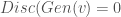$Disc(Gen(v)=0$ . In other word, the discriminator is designed to discriminate between the real c objects and the generated ones. Of course, if the Generator is really doing a good job of imitating then the discriminator with this condition would be very hard to build. In this case we would expect $Disc(Gen(v)=1$ .

Generative Adversarial networks

were introduced by Goodfellow et, al (arXiv:1406.2661) as a way to build neural networks that can generate very good examples that match the properties of a collection of objects. It works by designed two networks: one for the generator and one for the discriminator. Define to be the distribution of latent variables that the generator will map to the collection space. The idea behind the paper is to simultaneously design the discriminator and the generator as a two-player min-max game.

The discriminator is being trained to recognize object from c (thereby reducing for ) and pushing to zero for . The resulting function

Represents the min-max objective for the Discriminator.

On the other hand, the generator wants to push to 1 thereby maximizing
. To do that we minimize

There are literally dozens of implementations of GANs in Tensorflow or Karas on-line. Below is an example from one that works with 40×40 color images. This fragment shows the step of setting up the training optimization.

#These two placeholders are used for input into the generator and discriminator, respectively.
z_in = tf.placeholder(shape=[None,128],dtype=tf.float32) #Random vector
real_in = tf.placeholder(shape=[None,40,40,3],dtype=tf.float32) #Real images
Gz = generator(z_in) #Generates images from random z vectors
Dx = discriminator(real_in) #Produces probabilities for real images
Dg = discriminator(Gz,reuse=True) #Produces probabilities for generator images
#These functions together define the optimization objective of the GAN.
d_loss = -tf.reduce_mean(tf.log(Dx) + tf.log(1.-Dg)) #This optimizes the discriminator.
g_loss = -tf.reduce_mean(tf.log(Dg)) #This optimizes the generator.
tvars = tf.trainable_variables()
#The below code is responsible for applying gradient descent to update the GAN.
trainerD = tf.train.AdamOptimizer(learning_rate=0.0002,beta1=0.5)
trainerG = tf.train.AdamOptimizer(learning_rate=0.0002,beta1=0.5)

#Only update the weights for the discriminator network.
d_grads = trainerD.compute_gradients(d_loss,tvars[9:]) 
#Only update the weights for the generator network.
g_grads = trainerG.compute_gradients(g_loss,tvars[0:9]) 
update_D = trainerD.apply_gradients(d_grads)
update_G = trainerG.apply_gradients(g_grads)

We tested this with a very small collection of images of galaxies found on the web. There are three types: elliptical, spiral and barred spiral. Figure 4 below shows some high-resolution samples from the collection.

(Note: the examples in this section use pictures of galaxies, but , in terms of the discussion in the previous part of this article, these are illustrations only. There are no scientific results; just algorithm demonstrations. )

Figure 4. Sample high-resolution galaxy images

We reduced the images to 40 by 40 and trained the GAN on this very small collection. Drawing samples at random from the latent z-space we can now generate synthetic images. The images we used here are only 40 by 40 pixels, so the results are not very spectacular. As shown below, the generator is clearly able to generate elliptical and spiral forms. In the next section we work with images that are 1024 by 1024 and get much more impressive results.

Figure 5. Synthetic Galaxies produced by the GAN from 40×40 images.

Variational Autoencoders

The second general category generative models are based on variational autoencoders. An autoencoder transforms our collection of object representations into a space of much smaller dimension in such a way so that that representation can be used to recreate the original object with reasonably high fidelity. The system has an encoder network that creates the embedding in the smaller space and a decoder which uses that representation to regenerate an image as shown below in Figure 6.

Figure 6. Generic Autoencoder

In other words, we want to approximate for each i in an enumeration of our collection of objects. To train our networks we simply want to minimize the distance between and for each i. If we further set up the network inputs and outputs so that they are in the range [0, 1] we can model this as a Bernouli distribution so cross entropy is a better function to minimize. In this case the cross entropy can be calculated as

(see http://www.godeep.ml/cross-entropy-likelihood-relation/ for a derivation)

A variational autoencoder differs from a general one in that we want the generator to create an embedding that is very close to a normal distribution in the embedding space. The way we do this is to make the encoder force the encoding into a representation consisting of a mean and standard deviation. To force it into a reasonably compact space we will force our encoder to be as close to as possible. To do that we need a way to measuree how far a distribution p is from a Gaussian q. That is given by the Kullback-Leibler divergence which measures now many extra bits (or ‘nats’) are needed to convert an optimal code for distribution q into an optimal code for distribution p.

If both p and q are gaussian this is easy to calculate (thought not as easy to derive).

In terms of probability distributions we can think of our encoder as where x is a training image. We are going to assume is normally distributed and let be parameterized by . Computing is now easy. We call this the Latent Loss and it is

(see https://stats.stackexchange.com/questions/7440/kl-divergence-between-two-univariate-gaussians for a derivation).

We now construct our encoder to produce and . To sample from this latent space, we simply draw from and transform it into the right space. Our encoder and decoder networks can now be linked as follows.

the loss function is now the sum of two terms:

Note: there is a Baysian approach to deriving this. see https://jaan.io/what-is-variational-autoencoder-vae-tutorial for an excellent discussion.

One of the interesting properties of VAEs is that they do not require massive data sets to converge. Using our simple galaxy photo collection we trained a simple VAE. The results showing the test inputs and the reconstructed images are illustrated below.

Figure 7. test input and reconstruction from the galaxy image collection. These images are 1024×1024.

Using encodings of five of the images we created a path through the latent space to make the gif movie that is shown below. While not every intermediate “galaxy” looks as good as some of the originals, it does present many reasonable “synthetic” galaxies that are on the path between two real ones.

Figure 8. image from the “movie”

The notebook for this autoencoder is available as html (see https://s3.us-east-2.amazonaws.com/a-book/autoencode-galaxy.html) and as a jupyter notebook (see https://s3.us-east-2.amazonaws.com/a-book/autoencode-galaxy.ipynb ) The compressed tarball of the galaxy images is here: https://s3.us-east-2.amazonaws.com/a-book/galaxies.tar.gz.

acGANs

The generative networks described above are just the basic variety. One very useful addition is the Auxiliary Classifier GAN. An acGAN allows you to incorporate knowledge about the class of the objects in your collection into the process. For example, suppose you have labeled images such as all pictures of dogs are labeled “dog” and all pictures of cats have the label “cat”. The original paper on this subject “Conditional Image Synthesis with Auxiliary Classiﬁer GANs” by Oden, Olah and Shlens shows how a GAN can be modified so that the generator can be modified so that it takes a class label in addition to the random latent variable so that it generates a new element similar to the training examples of that class. The training is augmented with an additional loss term that models the class of the training examples.

There are many more fascinating examples. We will describe them in more detail in a later post.

The State of the Cloud for Science -2018

Introduction

This post is based on a talk I prepared for the Scientific Cloud Computing Workshop at HPDC 2018.

Two years ago, Ian Foster and I started writing “Cloud Computing for Science and Engineering”. That book covers fundamental cloud tools and computational models, but there are some topics we alluded to but did not explore fully because they were still on the horizon. In other cases, we were simply clueless about changes that were coming. Data center design and cloud services have evolved in some amazing ways in just two years and many of these changes represent opportunities for using cloud technology in scientific research.

Whose cloud?

Any discussion of cloud computing in science leads to the question of definition. What defines a cloud for science? For example, the European Open Science Cloud (EOSC) is a European-wide virtual environment for data sharing and collaboration. That project will involve multiple data archives, research labs and HPC centers, commercial service providers and EU agencies and funding. It is truly an important project. However, my focus here is on the fundamental technologies that are driving hardware and software innovation, and these tend to come from a combination of academic, open source and commercial providers. The most ubiquitous commercial clouds are:

Amazon Web Services (AWS) – 40% of all commercial cloud resources on the planet,
Microsoft Azure – about 50% of AWS but growing,
Google Cloud – a solid and growing third place,
IBM Bluemix – growing very fast and in some measures bigger now that Google.

There are many more, smaller or more specialized providers: Salesforce, DigitalOcean, Rackspace, 1&1, UpCloud, CityCloud, CloudSigma, CloudWatt, Aruba, CloudFerro, Orange, OVH, T-Systems.

There are a number of smaller cloud systems that have been deployed for scientific research. They include Aristotle, Bionimbus, Chameleon, RedCloud, indigo-datacloud, EU-Brazil Cloud, and the NSF JetStream. The advantage of these research clouds is that they can be optimized for use by a specific user community in ways not possible in a commercial cloud. For example, Chameleon is funded by the US NSF to support basic computer systems research at the foundational level which is not possible when the foundation is proprietary.

Are these clouds of any value to Science?

When the first commercial clouds were introduced in 2008 the scientific community took interest and asked if there was value there. In 2011 the official answer to this question seemed to be “no”. Two papers (see end node 1) described research experiments designed to address this question. The conclusion of both papers was that these systems were no match for traditional supercomputers for running MPI-based simulation and modeling. And, in 2010, they were correct. Early cloud data centers were racks of off-the-shelf PCs and the networks had terrible bisection bandwidth and long latencies. They were no match for a proper HPC cluster or supercomputer.

Over the last few years, others have recognized a different set of roles for the cloud in science that go beyond traditional supercomputer simulation. The biology community was quick to adopt cloud computing especially when it is necessary to do large scale analysis on thousands of independent data samples. These applications ranged from metagenomics to protein folding. These computations could each fit on a single server, so network bandwidth is not an issue and, using the scale of the cloud, it is easy to launch thousands of these simultaneously. Hosting and sharing large public scientific data collections is another important application. Google, AWS, Microsoft and other have large collections and they also are also providing new ways to host services to explore this data.

However, there are at least three additional areas where the cloud is a great platform for science.

Analysis of streaming data

Microsoft’s AI for earth project (Figure 1) looks at the application of streaming data from sources such as satellites to do land cover analysis, sensors on and above farm land to improve agriculture outcomes and crowd sourced data to help understand biodiversity.

Figure 1. Applications of streaming include land cover analysis, using sensor data for improving agriculture and biodiversity. From https://www.microsoft.com/en-us/aiforearth

The internet of things is exploding with sensor data as are on-line experiments of all types. This data will be aggregated in edge computing networks that do initial analysis with results fed to the cloud systems for further analysis. Urban Informatics is a topic that has emerged as critical to the survival of our cities and the people who live in them. Sensors of all types are being deployed in cities to help understand traffic flow, microclimates, local pollution and energy waste. Taken together this sensor data can paint a portrait of the city that planners can use to guide its future. Streaming data and edge computing is a topic that will involve the growing capabilities and architecture of the cloud. We will return to this later in this document.

Interactive big data exploration

Being able explore and interact with data is a critical component of science. If it fits on our laptop we can use tools like Matlab, Excel or Mathematica to conduct small computational experiments and visualize the results. If the data is too big it must be stored on something bigger than that laptop. Traditional supercomputers are up to the task of doing the analysis, but because they are designed around batch computing there are not well suited to interactive use. The cloud exists to host services that can be used by thousands of simultaneous users. In addition, there is a new generation of interactive data analysis tools that are cloud-ready for use on very large data collections. This collection of tools includes Spark and Python Dask. In both cases these tools can be driven by the open-source Jupyter studio which provides a powerful, interactive compute and visualization tool. The commercial providers have adapted Jupyter and its interactive computational model into their offerings. Google has Cloud Datalab (Figure 2), Amazon uses Jupyter with its SageMaker Machine Learning platform and Microsoft provide a special data science virtual machine that runs Jupyter Hub so that teams of users can collaborate.

Figure 2. Google’s Cloud Data lab integrates SQL-like queries to be combined with Python code and visualization to a Jupyter based web interface. https://cloud.google.com/datalab/

Being able to interact with data at scale is part of the power of the cloud. As this capability is combined with advanced cloud hosted machine learning tools and other services, some very promising possibilities arise.

The quest for AI and an intelligent assistant for research

The commercial clouds were originally built to host web search engines. Improving those search engines led to a greater engagement of the tech companies with machine learning. That work led to deep learning which enabled machine language translation, remarkably strong spoken language recognition and generation and image analysis with object recognition. Many of these capabilities rival humans in accuracy and speed. AI is now the holy grail for the tech industry.

One outcome of this has been the proliferation of voice-driven digital assistants such as Amazon’s Echo, Microsoft’s Cortana, Apple’s Siri and Google Assistant. When first introduce these were novelties, but as they have improved their ability to give us local information, do web searching, keep our calendars has improved considerably. I believe there is an opportunity for science here.

Ask the question “what would it take to make Alexa or Cortana help with my research?” The following use cases come to mind.

Provide a fast and accurate search of the scientific literature for a given specific scientific concept or topic and not just a keyword or specific author. Then ask who is working on or has worked on this topic? Is there public data in the cloud related to experiments involving this topic? Translate and transcribe related audio and video.
Understand and track the context of your projects.
Help formulate, launch and monitor data analysis workflows. Then coordinate and catalog results. If state-space search is involved, automatically narrow the search based on promising findings.
Coordinate meetings and results from collaborators.

If I ask Alexa to do any of this now, she would politely say “Sorry. I can’t help you with that.” But with the current rate of change in cloud AI tools, ten years seems like a reasonable timeframe.

Figure 3. Siri’s science geek grandson.

Technical Revolutions in the Cloud

Two of the three scenarios above are here now or very close. The third is some ways off. There have been three major changes in cloud technology in the past five years and some aspects of these changes are true game-changers for the industry. The first, and most obvious is the change in scale of cloud deployments. The two leaders, AWS and Azure are planetary in scale. This is illustrated in Figure 4 below.

Figure 4. A 2016 map of cloud coverage from Atomia.com. https://www.atomia.com/2016/11/24/ comparing-the-geographical-coverage-of-aws-azure-and-google-cloud/ There is some inaccuracy here because AWS and Azure define regional data centers differently, so counting the dots is not a good comparison. In addition, data centers are now under construction in South Africa and the Middle East.

This map does not include all the data centers run by the smaller cloud providers.

Cloud Services

A major departure from the early days of the cloud, where scientists focused on storage and servers, has been an explosion in pay-by-the-hour cloud hosted services. In addition to basic IaaS the types of services available now are:

App services: Basic web hosting, mobile app backend
Streaming data: IoT data streams, web log streams, instruments
Security services: user authentication, delegation of authorization, privacy, etc.
Analytics: database, BI, app optimization, stream analytics
Integrative: networking, management services, automation

In addition, the hottest new services are AI machine learning services for mapping, image classification, voice-to-text and text-to-voice services and text semantic analysis. Tools to build and train voice activated bots are also now widely available. We will take a look at two examples.

A planet scale database

The Azure Cosmos DB is a database platform that is globally distributed. Of course, distributing data across international boundaries is a sensitive topic, so the Cosmos platform allows the database creator to pick the exact locations you want copies to reside. When you create an instance of the database you use a map of Azure data centers and select the locations as shown in Figure 5.

Figure 5. Cosmos DB. A database created in central US and replicated in Europe, South India and Brazil.

The database can support 4 modes: Documents, key-value Graph and NoSQL. In addition, there are five different consistency models the user can select: eventual, consistent prefix, session, bounded stateless and strong consistency all with 99.9% guarantee of less than 15ms latency. My own experiments validated many these claims.

Cloud AI Services

The commercial clouds are in a race to see who can provide the most interesting and useful AI services on their cloud platform. This work began in the research laboratories in universities and companies over the past 25 years, but the big breakthroughs came when deep learning models trained on massive data collections began to reach levels of human accuracy. For some time now, the public cloud companies have provided custom virtual machines that make it easy for technically sophisticated customers to use state of the art ML and neural network tools like TensorFlow, CNTK and others. But the real competition is now to provide services for building smart applications that can be used by developers lacking advanced training in machine learning and AI. We now have speech recognition, language translation, image recognition capabilities that can be easily integrated into web and mobile applications.

We gave this a try with services that use a technique called Transfer Learning to make it possible to re-train a deep neural network to recognize objects from a narrow category using a very small training set. We chose images of galaxies and used the services of IBM Watson, Azure and Amazon. Figure 6 illustrates the results from IBM’s tool. The results were surprisingly good.

Figure 6. IBM’s Watson recognizing previously unseen images of three different galaxies. The details of this study are here: https://esciencegroup.com/2018/02/16/cloud-services-for-transfer-learning-on-deep-neural-networks/

The Revolution in Cloud Service Design

Making all of these services work, perform reliably and scale to thousands of concurrent users forced a revolution in cloud software design. In order to support these applications, the tech companies needed a way to design them so that they could be scaled rapidly and updated easily. They settled on a design pattern that based on the idea of breaking the applications into small stateless components with well defined interfaces. Statelessness meant that a component could be replaced easily if it crashed or needed to be upgraded. Of course, not everything can be stateless, so state is saved in cloud hosted databases. Each component was a “microservice” and it could be built from containers or functions. This design pattern is now referred to as “cloud native” design. Applications built and managed this way include Netflix, Amazon, Facebook, Twitter, Google Docs, Azure CosmosDB, Azure Event hub, Cortana, Uber.

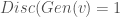
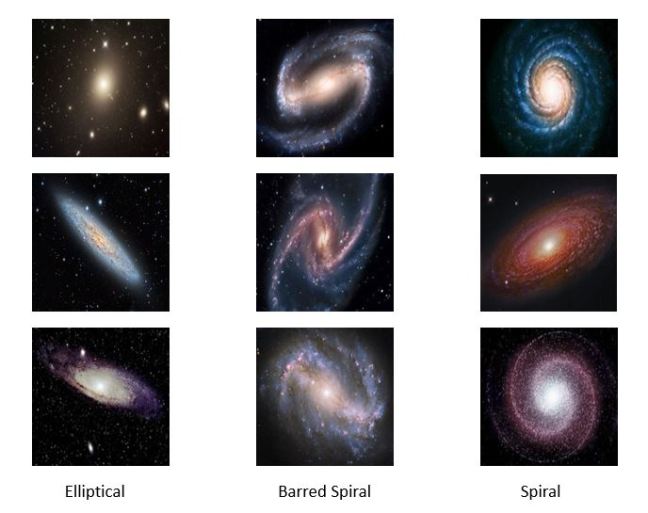
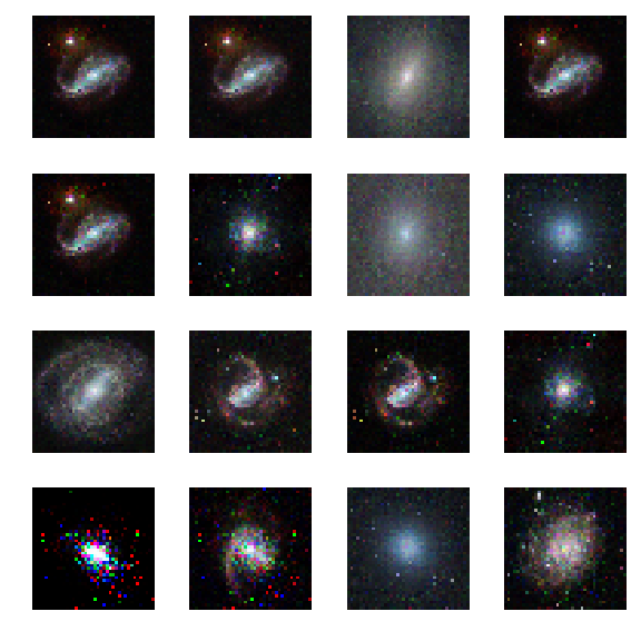
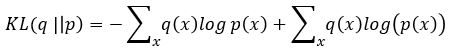
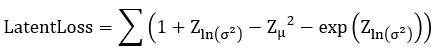
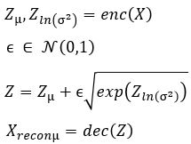
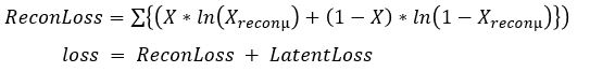
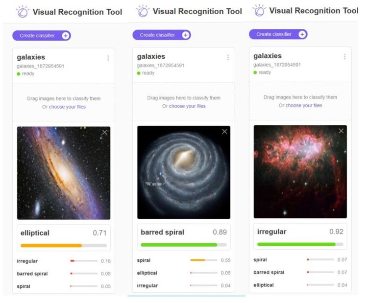
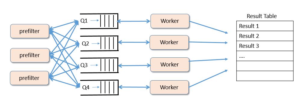
Figure 7. Conceptual view of microservices as stateless services communicating with each other and saving needed state in distribute databases or tables.

To manage applications that required dozens to hundreds of concurrently running microservice you need a software foundation or container orchestration system to monitor the services and schedule them on available resources. Several candidates emerged and are used. Siri, for example, is composed of thousands of microservices running on the Apache Mesos system. Recently cloud providers have settled on a de-facto standard container orchestrator built by Google and released as open source called Kubernetes. It is now extremely easy for any customer to use Kubernetes on many cloud deployments to launch and manage cloud native applications.

Serverless Functions

The next step in the cloud software evolution was the introduction of “serverless functions”. The original idea of cloud computing involved launching and managing a virtual machine. However, suppose you want to have a cloud-based application whose sole job is to wait for an event to trigger some action. For example, monitor a file directory and wait for a change such as the addition of a new file. When that happens, you want to send email to a set of users alerting them of the change. If this is a rare event, you don’t want to have to pay for an idle virtual machine that is polling some service looking for a change. Amazon was the first to introduce the concept of a function-as-a-service. With AWS Lambda, you only need to describe the function in terms of the trigger event and the output actions it takes when the even appears. As illustrated in Figure 8, there are many possible triggers and corresponding output channels.

Figure 8. From Amazon AWS. The triggers and outputs of a lambda function.

In addition to AWS Lambda, Azure Functions, Google Functions, IBM OpenWhisk are similar systems. OpenWhisk is now open source. Another open source solution is Kubeless that allow you to deploy a lambda-like system on top of your Kubernetes cluster. These serverless systems let you scale up and down extremely rapidly and automatically. You can have hundreds of instances responding to events at once. And the cost is based on charge-by-use models. AWS has introduced AWS Fargate which allows any containerized application to run in serverless mode.

The Edge and the Fog

The frontier of cloud computing is now at the edge of the network. This has long been the home of content distribution systems where content can be cached and access quickly, but now that the Internet-of-Things (IoT) is upon us, it is increasingly important to do some computing at the edge. For example, if you have a thousand tiny sensors in a sensitive environment or farm and you need to control water from sprinklers or detect severe weather conditions, it is necessary to gather the data, do some analysis and signal an action. If the sensors are all sending WIFI messages they may be routable to the cloud, but a more common solution is to provide local computing that can do some event preprocessing and response while forwarding summary data to the cloud. That local computing is called the Edge, or if a distributed systems of edge servers, the Fog.

If serverless functions are designed to respond to signals, that suggests that it should be possible to extend them to run in the edge servers rather than the cloud. AWS was the first to do this with a tool called GreenGrass that provides a special runtime system that allows us to push/migrate lambda functions or microservices from the data center to the edge. More recently Microsoft has introduced Azure IoT Edge which is built on open container technologies. Using an instance open source Virtual Kubelet deployed on the edge devices we can run our Kubernetes containers to run on the edge. You can think of a Kubelet as the part of Kubernetes that runs on a single node. This enables Kubernetes clusters to span across the cloud and edge as illustrated in Figure 9.

Figure 9. shows a sketch of migrating containerized functions to edge function. That way our IOT devices can communicate with locally deployed microservices. These microservices can communicate with cloud-based services. The edge function containers can also be updated and replaced remotely like any other microservice.

The Evolution of the Data Center

As mentioned at the beginning of this paper, the early days (2005) of cloud data center design systems were based on very simple server and networks were designed for outgoing internet traffic and not bisectional bandwidth for parallel computing. However, by 2008 interest in performance began to grow. Special InfiniBand sub-networks were being installed at some data centers. The conventional dual-core servers were being replaced by systems with up to 48 cores and multiple GPU accelerators. By 2011 most of the commercial clouds and a few research clouds had replaced traditional network with software defined networking. To address the demand of some of its customers, in 2017 Microsoft added Cray® XC™ and Cray CS™ supercomputers to a few data centers and then acquired the company cycle computing.

From 2016 we have seen progress focused on performance and parallelism. The driver of this activity has been AI and, more specifically, the deep neural networks (DNNs) driving all the new services. There are many types of DNNs but two of the most common are convolutional, which look like a linear sequence of special filters, and recurrent networks which, as the name implies, are networks with a feedback component. And there are two phases to neural network design and use. The first is the training phase which requires often massive parallelism and time. But it is usually an off-line activity. The second phase is called inference and it refers to the activity of evaluating the trained network on classification candidates. In both the convolutional and recurrent network inference boils down to doing a very large number of matrix-vector and matrix-matrix multiplies where the coefficients of the matrix are the trained model and the vector represent the classification candidates. To deliver the performance at scale that was needed by the AI services it was essential to do these operations fast. While GPUs were good, more speed was needed.

Google’s Tensor Processing Unit

In 2015 Google introduced the Tensor Processing Unit (TPU) and the TPU2 in 2017.

Figure 10. Above, Google data center. https://www.nextplatform.com/2017/05/22/hood-googles-tpu2-machine-learning-clusters/ Below architecture of Google Tensor Processing Unit TPU. From “In-Datacenter Performance Analysis of a Tensor Processing Unit”, Norman P. Jouppi et al. ISCA 2017 https://ai.google/research/pubs/pub46078

Figure 10 illustrates several racks of TPU equipped servers and the functional diagram of the TPU. One of the key components is the 8-bit matrix multiply capable of delivering 92 TeraOps/second (TOPS). (It should be noted that DNNs can be well trained on less than IEEE standard floating-point standards and floating point systems with small mantissa are popular.) The multiply unit uses a systolic algorithm like those proposed for VLSI chips in the 1980s.

Microsoft’s Brainwave

In 2011 a small team in Microsoft Research led by Doug Burger began looking at the use of FPGAs to accelerate the search result ranking produced by Bing. Over several iterations they arrived at a remarkable design that allowed them to put the FPGA between the network and the NIC so that the FPGA could be configured into separate plane of computation that can be managed and used independently from the CPU (see Figure 11). Used in this way groups of FPGAs could be configured into a subnetwork to handle tasks such as, database queries and inference stage of deep learning in addition to Bing query optimization.

Figure 11. The Brainwave architecture.

Figure 12. The brainwave software stack for mapping a DNN to one or more FPGAs. From BrainWave_HOTCHIPS2017.pptx, Eric Chung, et. al., https://vneetop.wordpress.com/ 2017/10/28/accelerating-persistent-neural-networks-at-datacenter-scale/

The team also built a software stack that could really make this possibility a reality. What makes much of this possible is that the models for DNNs are all based on flow graphs which describe sequences of tensor operations. As shown in Figure 12 above, the flow graphs can be compiled to a graph internal representation that can be split and partitioned across one or more FPGAs. They refer to the result as a hardware microservice. Just recently Mary Wall [see endnote 2] wrote a nice blog about the teams work on using this idea to do deep learning inference on land cover maps. Each compiled inference hardware microservice is mapped to a single FPGA, but they used 800 of the inference instances in parallel with 80 VMs to process 20 terabytes of aerial imagery into land cover data for the entire United States. It took only about 10 minutes for a total cost of $42. [see endnote3] Mary Wall’s code is in the blog and available in Github.

Conclusion

Cloud data centers are getting high performance networks (with latencies of only a few microseconds in the case of Azure Brainwave) and immense computing capacity such as the tensor processing capability of Google’s TPU. At the same time designers of supercomputers are having to deal with more failure resilience and complexity in the design of the first exascale supercomputers. For the next generation exascale systems the nodes will be variations on a theme of multicore and GPU-style accelerators.

Observed from a distance, one might conclude the architectures of cloud data centers and the next generation of supercomputers are converging. However, it is important to keep in mind that the two are designed for different purposes. The cloud is optimized for fast response for services supporting many concurrent globally distributed clients. Supers are optimized for exceptionally fast execution of programs on behalf of a small number of concurrent users. However, it may be the case that an exascale system may be so large that parts of it can run many smaller parallel jobs at once. Projects like Singularity provide a solution for running containerized application on supercomputers in a manner similar to the way microservices are run on a cloud.

Possible Futures

The continuum: edge+cloud+supercomputer

There are interesting studies showing how supercomputers are very good at training very large, deep neural networks. Specifically, NERSC scientists have show the importance of this capability in many science applications[4]. However, if you need to perform inference on models that are streamed from the edge you need the type of edge+cloud strategy described here. It not hard to imagine scenarios where vast numbers of instrument streams are handled by the edge and fed to inference models on the cloud and those models are being continuously improved on a back-end supercomputer.

A data garden

In the near future, the most important contribution clouds can make to science is to provide access to important public data collections. There is already reasonable start. AWS has an opendata registry that has 57 data sets covering topics ranging from astronomy to genomics. Microsoft Research has a Data Science for Research portal with a curated collection of datasets relating to human computer interaction, data mining, geospatial, natural language processing and more. Google cloud has a large collection of public genomics datasets. The US NIH has launch three new cloud data and analytics projects. They include the Cancer Genomics Cloud led by the Institute for Systems Biology with Google’s cloud, FireCloud from the Broad Institute also using Google’s cloud and Cancer Genomics Cloud (CGC), powered by Seven Bridges. These NIH facilities also provide analytics frameworks designed to help research access and effective use the resources.

I am often asked about research challenges in cloud computing that student may wish to undertake. There are many. The fact that the IEEE cloud computing conference being held in San Francisco in July received nearly 300 submissions shows that the field is extremely active. I find the following topics very interesting.

Find new ways to extract knowledge from the growing cloud data garden. This is a big challenge because the data is so heterogeneous and discovery of the right tool to use to explore it requires expert knowledge. Can we capture that community knowledge so that non-experts can find their way? What are the right tools to facility collaborative data exploration?
There are enormous opportunities for systems research in the edge-to-cloud-to-supercomputer path. How does one create a system to manage and optimize workflows of activities that span this continuum? Is there a good programming model for describing computations involving the edge and the cloud? Can a program be automatically decomposed into the parts that are best run on the edge and the parts on cloud? Can such a decomposition be dynamically adjusted to account for load, bandwidth constraints, etc.?
Concerning the intelligent assistant for research, there are a number of reasonable projects short of build the entire thing. Some may be low hanging fruit, and some may be very hard. For example, ArXiv, Wikipedia and Google search and Bing are great for discovery but in different ways. Handling complex queries like “what is the role of quantum entanglement in the design of a quantum computer?” should lead to a summary of the answer with links. There is a lot of research on summarization and there are a lot of sources of data. Another type of query is “How can I access data on genetic indicators related to ALS?” Google will go in the right direction, but it takes more digging to find data.

These are rather broad topics, but progress on even the smallest part may be fun.

[1] L. Ramakrishnan, P. T. Zbiegel, S. Campbell, R. Bradshaw, R. S. Canon, S. Coghlan, I. Sakrejda, N. Desai, T. Declerck, and A. Liu. Magellan: Experiences from a science cloud. In 2nd International Workshop on Scientiﬁc Cloud Computing, pages49–58., ACM, 2011.

P. Mehrotra, J. Djomehri, S. Heistand, R. Hood, H. Jin, A. Lazanoﬀ, S. Saini, and R. Biswas. Performance evaluation of Amazon EC2 for NASA HPC applications. In 3rd Workshop on Scientiﬁc Cloud Computing, pages 41–50. ACM, 2012

[2] https://blogs.technet.microsoft.com/machinelearning/2018/05/29/how-to-use-fpgas-for-deep-learning-inference-to-perform-land-cover-mapping-on-terabytes-of-aerial-images/ a blog by Mary Wall, Microsoft

[3] https://blogs.microsoft.com/green/2018/05/23/achievement-unlocked-nearly-200-million-images-into-a-national-land-cover-map-in-about-10-minutes/ from Lucas Joppa – Chief Environmental Scientist, Microsoft

[4] https://www.hpcwire.com/2018/03/19/deep-learning-at-15-pflops-enables-training-for-extreme-weather-identification-at-scale/

Algorithmia™: A Cloud Marketplace for Algorithms and Deep Learning

One area of great frustration encountered by application developers involves the challenge of integrating new algorithms into a code base. There are many reasons for this. For example, the algorithm may be described in a journal article where many details of the implementation are omitted or it is available only in a programming language different from the one being used. The code may have software dependencies that are hard to resolve. The new algorithm may also have hardware dependencies, such as reliance on a GPU to get performance and you may not have access to this hardware. On the other hand, if you are the author of a great new algorithm you may be disappointed that your new invention is not being used for these very same reasons.

About 18 months ago a company called Algorithmia™ was founded in Seattle that provides an elegant solution to these problems. They provide a very simple multi-language API that can be used to invoke any of their catalog of 3,500 different cloud-based algorithms. While we may be getting tired of reading about X-as-a-Service for different versions of X, there is one binding for X that has been around for a while in various forms and, as much as it pains me to do so, it begs to be called Algorithms as a Service. And AaaS is just one of the things Algorithmia provides.

AaaS is indeed not a new idea. Jack Dongarra and his ICL team at the University of Tennessee created NetSolve/GridSove in 2003 to provide scientists and engineers with access to state-of-the-art numerical algorithms running on a distributed network of high performance computers. As cool as NetSolve is, Algorithmia goes several steps beyond this concept.

One of Algorithmia’s cofounders and CEO, Diego Oppenheimer has a deep background in building business intelligence tools. While working on that he developed an appreciation of the power of being able to call out to powerful algorithms from inside a user facing application. This capability allows the application to have access to deeper knowledge and more powerful computational resources than available on the user’s device. A key insight from this experience is that algorithms must be discoverable an invokable from any user application runtime. These ideas are all central to Algorithmia. In the following paragraphs we will look at Algoritmia’s marketplace, explore building a new algorithm and discuss a bit of the system microservice architecture.

Algorithmia is a marketplace.

There are over 50,000 developers that use Algorithmia services and the platform encourages these developers to contribute new algorithms to the collection. Invoking an algorithm is dead simple and it can be done from any programming language that can formulate a JSON doc and send a REST message. We will provide some detailed illustrations at the end of this document.

To use it, you need to set up an account. Doing so will get you a starter award of 5000 or so “credits”. When you invoke an algorithm, credits are deducted from your account. Typically, there is a “royalty” cost of about 10 credits and then the cost is usually around one credit per second of execution. A fun example from their library of deep learning collection is an image colorizer. Input is a PNG file of a black and white image and the returned value is a link to the output colorized image. We took a color image from a visit to Red Square a few years ago. We converted it to a grayscale image and gave that to the colorizer. The result is shown illustrated below. The original is on the left, grayscale in the middle and the colorized image on the right. While it is not as good as the best hand-colored photos, it is not too bad. It lost the amazing color of St. Bazil’s Cathedral which is not too surprising, but it was great with sky and skin tones of those people in foreground. (It seemed to think the bricks of the square would look better with some grass color.)

colorized

The Python code to upload the grayscale image and invoke the service was incredibly simple.

import Algorithmia
client = Algorithmia.client(‘youruserkeyfromaccountrecation’)
input = bytearray(open("path_to_grayscale.png", "rb").read())
result = client.algo("deeplearning/ColorfulImageColorization/1.1.6")
        .pipe(input).result
path_to_local_copy_of_result_image= client.file(result[‘output’]).getFile()

The cost in credits was 154. The exchange rate for credits is 1$ = 10,000 credits (approximately) so this invocation would have cost about 1.5 cents.

This algorithm is from their extensive machine learning and AI collection. A related algorithm is one that computes the salience of objects in an image. Salience is the degree to which an object in the image attracts the attention of the viewer’s eye. The algorithm is called SalNet and it is based on ideas from the paper, Shallow and Deep Convolutional Networks for Saliency Prediction by Pan et. al. (see arXiv:1603.00845v1).

As with the colorizer, salnet it is easy to invoke.

input = { "image": "data://.algo/deeplearning/SalNet/perm/an-uploaded-image.png" }
result2 = client.algo("deeplearning/SalNet/0.2.0").pipe(input).result

Note that in this case we have loaded the image from one that we uploaded to Algorithmia’s data cloud. In fact, it is the same grayscale image of red square. As you can see below, the algorithm picks out the woman in the foreground and also notices the church in the background.

Salience computation can be very helpful in identifying and labeling objects in an image. Image tagging is also something that Algorithmia supports. Running the same image through their tagger returned the observations that the image was “safe” and that there were multiple boys and multiple girls and sky and clouds and it seem to be near a palace.

salience2

There are many other AI related image algorithms such as nudity detection, character recognition, face detection and a very impressive car make and model recognition algorithm. A quick look at https://algorithmia.com/use-cases will show many other fascinating use cases.

Another very cool capability of Algorithmia is its ability to host your trained machine learning model. Suppose you have a model you have built with MsXNet, TensorFlow, Scikit-Learns, CNTK or any of the other popular ML frameworks, you can upload your model to Algorithmia so that it can be available as a service. This is explained in here. We will explore this capability in a later post.

While the main emphasis and attraction of the Algorithmia collection is machine learning and AI, there are many more algorithm categories represented there. For example, there is an excellent collection of utilities for managing data and making certain programming tasks extremely easy: such as extracting text from web pages, Wikipedia search tools, computing the timezone and elevation from lat, lon coordinates.

There is also a large collection of time series analysis algorithms. These include forecasting, outlier detection, Fourier filters, auto-correlation computation and many more.

Algorithmia is cloud of microservices

In an excellent talk at the 2017 Geekwire cloud summit, Oppenheimer described some key elements of Algorithmia’s architecture. In this talk he makes the critically important observation that two phases of machine learning, training and prediction, if used in production require very different execution environments. Training is often done on a dedicated system consuming many hours of compute and as much memory as is available. The result of training is a model codified as data. Prediction (also called Inference) uses the model to make predictions or inferences about a sample case. Prediction can be done on the same hardware platform that was used for the training, but if the model is to be used to make predictions concerning thousands of cases for thousands of concurrent users, one need a completely different design.

Their approach to the scale problem for predictions (and for any high demand algorithm in their collection) is based on serverless microservices. They use a Kubernetes microservice foundation with algorithms deployed in Docker containers. Requests from remote client applications are load balanced across API servers who dispatch requests to container instances for the requested function. The challenge is making the latency from request to reply very low. If a container for an algorithm is already in system memory, it requires very little time to spawn a new instance on Kubernetes. Another technique they use it to dynamically load algorithms into running containers. (We don’t know the exact mechanism Algorithmia uses here, but we expect it is exploiting these facts.)

They have made some very interesting optimizations. For example, if the data used in the computation is stored in one of their cloud regions, the docker instance will be instantiated nearby. Just as important, if an algorithm invokes another algorithm they will attempt to co-locate the two containers and reduce the inter-process latency. Composability of algorithms is one of their guiding concepts.

Turning your own algorithm into a microservice.

The process of turning your own algorithm into a microservice is remarkably simple. From the Algorithmia portal there is a “+” symbol in the upper right-hand corner. This give you a dialog box to fill out. You provide a name of your algorithm, the programming language you are using (from a long list .. but sorry, no Fortran or Julia but there are lots of alternatives), and several other choices including: your source license policy, does your function invoke other Algorithmia functions, does your function invoke things on the open internet?

Answering these questions causes Algorithmia to create a nice GitHub repo for your function. Your next step is to install the Algorithmia command line interface and then you can clone your functions GitHub repo. Once you have done that you can edit the function so that it does what you want. The basic skeleton is already there for you in the “src” directory. Here is the basic skeleton in Python rendered as a hello world function.

import Algorithmia
# API calls will begin at the apply() method, 
# with the request body passed as 'input'
# For more details, see algorithmia.com/developers/algorithm- 
# development/languages
def apply(input):
    return "hello {}".format(input)

You can edit the function directly from an editor built into the Algorithmia portal or, now that you have a clone of the repo you can use your own tools to transform this skeleton into your algorithm. If you have done this work on your clone you need to use the Github commands to push your code back to the master.

We tried this with a small experiment. We built a function called KeyPhrases that takes English language text as input and breaks it down into subjects (s), actions (a) which are like verb clauses and objects (o). The algorithm is not very useful or sophisticated. In fact, it uses another Algorithmia microservice called Parsey McParseface which was originally released by Goolge (see https://arxiv.org/ pdf/1603.06042v1.pdf) . This is truly a deep parser that build a very sophisticated tree. For example the figure below illustrates the tree for a pars of the sentence

Einstein’s general theory of relativity explains gravity in terms of the curvature of spacetime.

parsey-einstein

Parsey McParseface tree output.

Our function KeyPhrases walks the tree and groups the terms, subjects(s), objects(o) and actions (a) and returns a JSON document with the original string and the list of phrases. It also breaks out separate subphrases with “/” marks. In this case it returns

{"phrases":[
       "s: Einstein's general theory /of relativity ",
       "a: explains ",
       "s: gravity /in terms /of the curvature /of spacetime. "
        ],
  "text":"Einstein's general theory of relativity explains gravity in terms of the curvature of spacetime."
}

A more complex example is

Facebook Incs chief security officer warned that the fake news problem is more complicated to solve than the public thinks.

The phrase output is

['s: Facebook Incs chief security officer ',
 'a: warned ',
 'o: that the fake news problem ',
 'a: is more ',
 'o: complicated and dangerous /to solve /than the public thinks ']

This is clearly not as rich in detail as the Parsey output, but it does extract some useful key phrases.

To complete the creation of the microservice for this algorithm one need only issue the git commands

$ git add src/KeyPhrases.py
$ git commit -m "added src mods"
$ git push origin master

The last push causes a compile step to happen and the microservice is now created. Algorithmia also provides an easy template to add documentation and instructions about how to invoke your function. From the Algorithmia editor there is a function that allows you to “publish” your algorithm. After pushing that button, the KeyPhrase example was put in their library. You can see it here: https://algorithmia.com/algorithms/dbgannon/KeyPhrases (If you use it, remember it has not been tested very well, so it may break.)

Algorithmia as an enterprise platform

The Algorithmia serverless microservice platform is robust enough that they offer it as an enterprise product. This allows enterprises to host their own version on one of the public clouds or on their own clusters or across multiple cloud in a hybrid system. This allows their own internally used algorithm to be hosted and invoked by their in-house analytics tools and pipelines in a totally scalable way. This enterprise version comes with a management dashboard and monitoring tools.

Conclusions

Algorithmia is a fascinating company with very interesting products. It is extremely easy to sign up for a free account and it is fun to use. The team was extremely helpful when we had questions. A Jupyter Notebook with some of the examples mentioned above will be posted very soon. We found experimenting with the various algorithms from an interactive notebook was a pleasure. Creating the hosted version of the KeyPhrases algorithm took less than an hour after the original python code was debugged. In our next experiment we will explore hosting deep learning models with Algorithmia.

CNTK Revisited. A New Deep Learning Toolkit Release from Microsoft

2 Replies

In a pair of articles from last winter (first article, second article) we looked at Microsoft’s “Computational Network Toolkit” and compared it to Google’s Tensorflow. Microsoft has now released a major upgrade of the software and rebranded it as part of the Microsoft Cognitive Toolkit. This release is a major improvement over the initial release. Because these older articles still get a fair amount of web traffic we wanted to provide a proper update.

There are two major changes from the first release that you will see when you begin to look at the new release. First is that CNTK now has a very nice Python API and, second, the documentation and examples are excellent. The core concepts are the same as in the initial release. The original programming model was based on configuration scripts and that is still there, but it has been improved and renamed as “Brain Script”. Brain Script is still an excellent way to build custom networks, but we will focus on the Python API which is very well documented.

Installing the software from the binary builds is very easy on both Ubuntu Linux and Windows. The process is described in the CNTK github site. On a Linux machine, simply download the gziped tared binary and execute the installer.

$wget https://cntk.ai/'BinaryDrop/CNTK-2-0-beta2-0-Linux-64bit-CPU-Only.tar.gz’
$tar -xf CNTK-2-0-beta2-0-Linux-64bit-CPU-Only.tar.gz
$cd cntk/Scripts/linux
$./install-cntk.sh

This will install everything including a new version of Continuum’s Anaconda Python distribution. It will also create a directory called “repos’’. To start Jupyter in the correct conda environment do the following.

$source “your-path-to-cntk/activate-cntk"
$cd ~/repos/cntk/bindings/python/tutorials
$Jupyter notebook

A very similar set of commands will install CNTK on your Windows 10 box. (If you are running Jupyter on a virtual machine or in the cloud you will need additional arguments to the Jupyter notebook command such as “-ip 0.0.0.0 –no browser” and then then you can navigate you host browser to the VM ip address and port 8888. Of course, if it is a remote VM you should add a password. ) What you will see is an excellent set of tutorials as shown in Figure 1.

Figure 1. CNTK tutorial Jupyter notebooks.

CNTK Python API

CNTK is a tool for building networks and the Python and Brain Script bindings are very similar in this regard. You use the Python program to construct a network of tensors and then train and test that network through special operations which take advantage of underlying parallelism in the hardware such as multiple cores or multiple GPUs. You can load data into the network through Python Numpy arrays or files.

The concept of constructing a computation graph for later execution is not new. In fact, it is an established programming paradigm used in Spark, Tensorflow, and Python Dask. To illustrate this in CNTK consider the following code fragment that creates two variables and a constructs a trivial graph that does matrix vector multiplication and vector addition. We begin by creating three tensors that will hold the input values to the graph and then tie them to the matrix multiply operator and vector addition.

import numpy as np
import cntk
X = cntk.input_variable((1,2))
M = cntk.input_variable((2,3))
B = cntk.input_variable((1,3))
Y = cntk.times(X,M)+B

In this X is a 1×2 dimensional tensor, i.e. a vector of length 2 and M is a matrix that is 2×3 and B is a vector of length 3. The expression Y=X*M+B yields a vector of length 3. However, no computation has taken place. We have only constructed a graph of the computation. To invoke the graph we input values for X, B and M and then apply the “eval’’ operator on Y. We use Numpy arrays to initialize the tensors and supply a dictionary of bindings to the eval operator as follows

x = [[ np.asarray([[40,50]]) ]]
m = [[ np.asarray([[1, 2, 3], [4, 5, 6]]) ]]
b = [[ np.asarray([1., 1., 1.])]]

print(Y.eval({X:x, M: m, B: b}))
array([[[[ 241.,  331.,  421.]]]], dtype=float32)

CNTK has several other important tensor containers but two important ones are

Constant(value=None, shape=None, dtype=None, device=None, name=”): a scalar, vector or other multi-dimensional tensor.
Parameter(shape=None, init=None, dtype=None, device=None, name=”): a variable whose value is modified during network training.

There are many more tensor operators and we are not going to go into them here. However, one very important class is the set of operators that can be used to build multilevel neural networks. Called the “Layers Library’’ they form a critical part of CNTK. One of the most basic is the Dense(dim) layer which creates a fully connected layer of output dimension dim. As shown in Figure 2.

Figure 2. A fully connected layer created by the Dense operator with an implicit 3×6 matrix and a 1×6 vector of parameters labeled here M and B. The input dimension is taken from the input vector V. The activation here is the default (none), but it could be set to ReLu or Sigmod or another function.

There are many standard layer types including Convolutional, MaxPooling, AveragePooling and LSTM. Layers can also be stacked with a very simple operator called “sequential’’. Two examples taken directly from the documentation is a standard 4 level image recognition network based on convolutional layers.

with default_options(activation=relu):
    conv_net = Sequential ([
        # 3 layers of convolution and dimension reduction by pooling
        Convolution((5,5), 32, pad=True), MaxPooling((3,3), strides=(2,2)),
        Convolution((5,5), 32, pad=True), MaxPooling((3,3), strides=(2,2)),
        Convolution((5,5), 64, pad=True), MaxPooling((3,3), strides=(2,2)),
        # 2 dense layers for classification
        Dense(64),
        Dense(10, activation=None)
    ])

The other fun example is a slot tagger based on a recurrent LSTM network.

tagging_model = Sequential ([
    Embedding(150),         # embed into a 150-dimensional vector
    Recurrence(LSTM(300)),  # forward LSTM
    Dense(labelDim)         # word-wise classification
])

The Sequential operator can be thought of as a concatenation of the layers that in the given sequence. In the case of the slot tagger network, we see two additional important operators: Embedding and Recurrence.

Embedding is used for word embeddings where the inputs are sparse vectors of size equal to the word vocabulary (item i = 1 if the word is the i-th element of the vocabulary and 0 otherwise) and the embedding matrix is of size vocabulary-dimension by, in this case, 150. The embedding matrix may be passed as a parameter or learned as part of training.

The Recurrence operator is used to wrap the correct LSTM output back to the input for the next input to the network.

A Closer Look at One of Tutorials.

The paragraphs above are intended to give you the basic feel of what CNTK looks like with its new Python interface. The best way to learn more is to study the excellent example tutorials.

CNTK 203: Reinforcement Learning Basics

CNTK version 1 had several excellent tutorials, but version 2 has the Python notebook versions of these plus a few new ones. One of the newest demos is an example of reinforcement learning. This application of Neural Nets was first described in the paper Human-level control through deep reinforcement learning, by the Google DeepMind group. This idea has proven to be very successful in systems that learn to play games. This topic has received a lot of attention, so we were happy to see this tutorial included in CNTK. The example is a very simple game that involves balancing a stick. More specifically they use the cart-pole configuration from OpenAI. As shown in figure 3, the system state can be described by a 4-tuple: position of the cart, its velocity, the angle of the pole and the angular velocity. The idea of the game is simple. You either push the cart to the left or the right and see if you can keep the stick vertical. If you drift too far off course or the pole angle goes beyond an angle of 15 degrees, the game is over. Your score is the total number of steps you take before failure. The full example is in the github repository and we are not going to go through all the code here. The Jupyter notebook for this example is excellent, but if you are new to this topic you may find some additional explanation of value in case you decide to dig into it.

Figure 3. Cart-Pole game configuration.

The part of reinforcement learning used here is called a Deep Q-Network. It uses a neural network to predict the best move when the cart is in a given state. This is done by implicitly modeling a function Q(s,a) which is the optimal future reward given state s and the action is a and where the initial reward is r. They approximate Q(s,a) using the “Bellmann equation” which describes how to choose action a in a given state s to maximize the accumulated reward over time based inductively on the same function applied to the following states s’.

The parameter gamma is a damping factor that guarantees the recurrence converges. (Another excellent reference for this topic is the blog by Jaromír Janisch.) The CNTQ team approached this problem as follows. There are three classes.

Class Brain. This hold our neural net and trainer. There are three methods
- Create() which is called at initialization. It creates the network. There are two tensor parameters: observation, which is used to hold the input state and q_target which is a tensor used for training. The network is nice and simple:
```
l1 = Dense(64, activation=relu)
l2 = Dense(2)
unbound_model = Sequential([l1, l2])
model = unbound_model(observation)
```
  The training is by the usual stochastic gradient descent based on a loss measure.
```
loss = reduce_mean(square(model - q_target), axis=0)
meas = reduce_mean(square(model - q_target), axis=0)
learner = sgd(model.parameters, lr,    
       gradient_clipping_threshold_per_sample=10)
trainer = Trainer(model, loss, meas, learner)
```
- Train(x, y) which calls the trainer for batches of states x and predicted outcomes y which we will describe below
- Predict(s) which invokes the model for state ‘s’ and returns a pair of optimal rewards given a left or right move.
Class Memory. This hold a record of recent moves. This is used by the system to create training batches. There are two methods
- Add(sample configuration) – adds a four tuple consisting of a starting state, an action and a result and a resulting state tuple to a memory.
- Sample(n) returns a random sample of n configurations samples from the memory.
Class Agent which is the actor that picks the moves and uses the memory to train the network. There are three methods here.
- Act(state) returns a 0 or 1 (left move or right move) that will give the best reward for the given state. At first it just makes random guesses, but as time passes it uses the Predict method of the Brain class to select the best move for the given state.
- Observe(sample configuration) records a configuration in the memory and keeps track of the time step and another parameter used by act.
- Replay() is the main function for doing the learning. This is the hardest part to understand in this tutorial. It works by grabbing a random batch of memorized configurations from memory. What we will do is use the current model to predict an optimal outcome and use that as the next step in training the model. More specifically for each tuple in the batch we want to turn it into a training sample so that the network behaves like the Bellmann equation. A tuple consists of the start state, the action, the reward and the following state. We can apply our current model to predict the award for the start state and also for the result state. We can use this information to create a new reward tuple for the given action and start state that models the Bellmann recurrence. Our training example is the pair consisting of the start state and this newly predicted reward. At first this is a pretty poor approximation, but amazingly over time it begins to converge. The pseudo code is shown below.
```
x = numpy.zeros((batchLen, 4)).astype(np.float32)
y = numpy.zeros((batchLen, 2)).astype(np.float32)

for i in range(batchLen):
    s, a, r, s_ = batch[i]
    # s = the original state (4 tuple)
    # a is the action that was taken
    # r is the reward that was given
    # s_ is the resulting state.
    # let t = the reward computed from current network for s 
    # and let r_ be the reward computed for state s_.
    # now modify t[a] = r + gamma* numpy.amax(r_) 
    # this last step emulated the bellmann equation
    x[i] = s
    y[i] = t
self.brain.train(x,y)		
```

The final part of the program is now very simple. We have an environment object that returns a new state and a done flag for each action the agent takes. We simply run our agent until it falls out of bounds (the environment object returns done=True). If the step succeeded, we increment our score. The function to run the agent and to keep score is shown below.

def run(agent):
    s = env.reset()
    R = 0 
    while True:            
        a = agent.act(s)
	  s_, r, done, info = env.step(a)
        if done: # terminal state
            s_ = None
        agent.observe((s, a, r, s_))
        agent.replay() #learn from the past           
        s = s_
        R += r
        if done:
            return R

Each time we run “run” it learns a bit more. After about 7000 runs it will take over 600 steps without failure.

The text above is no substitute for a careful study of the actual code in the notebook. Also, as it is a notebook, you can have some fun experimenting with it. We did.

Final Thoughts

CNTK is now as easy to use as any of the other deep learning toolkits. While we have not benchmarked its performance they claim it is extremely fast and it make good use of multiple GPUs and even a cluster of servers. We are certain that the user community will enjoy using and contributing to its success.

Citation.

The team that first created CNTK should be cited. I know there are likely many others that have contributed to the open source release in one way or another, but the following is the master citation.

Amit Agarwal, Eldar Akchurin, Chris Basoglu, Guoguo Chen, Scott Cyphers, Jasha Droppo, Adam Eversole, Brian Guenter, Mark Hillebrand, T. Ryan Hoens, Xuedong Huang, Zhiheng Huang, Vladimir Ivanov, Alexey Kamenev, Philipp Kranen, Oleksii Kuchaiev, Wolfgang Manousek, Avner May, Bhaskar Mitra, Olivier Nano, Gaizka Navarro, Alexey Orlov, Hari Parthasarathi, Baolin Peng, Marko Radmilac, Alexey Reznichenko, Frank Seide, Michael L. Seltzer, Malcolm Slaney, Andreas Stolcke, Huaming Wang, Yongqiang Wang, Kaisheng Yao, Dong Yu, Yu Zhang, Geoffrey Zweig (in alphabetical order), “An Introduction to Computational Networks and the Computational Network Toolkit“, Microsoft Technical Report MSR-TR-2014-112, 2014.

Azure Container Services Are Now Live: An Initial Look

1 Reply

The Microsoft Azure container services are now live and, for the most part, they work very well. There are actually two container services the Azure team is supporting. One is Mesosphere DC/OS and the other is Docker swarm. I have been using various versions of Mesos and Mesosphere for a year now, but those deployments were somewhat ad hoc. Some previous postings are here and here and this article provides some updates to both. These services are now in “general availability”, which is Microsoft speak for “it is now a product”. There is a good start-up tutorial available here which will lead you through the setup phase. In this post we will focus on some basic features of DC/OS and show a very simple example of how well it scales. In a future post we will look at Swarm.

DC/OS

Following the introduction tutorial lined above it was relatively easy to create a DC/OS cluster with 8 worker nodes (and one public node) and one master. Using the instructions, we also created a secure tunnel to the master node mapping port 80 there to localhost port 80. The web link http://localhost on my windows10 box brought up the DC/OS web user interface. What you see is the summary of all of the resources used as shown in Figure 1 below.

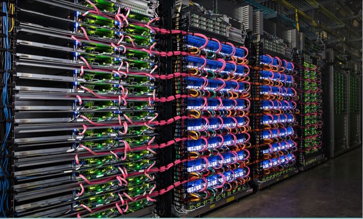
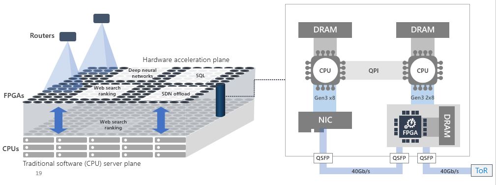
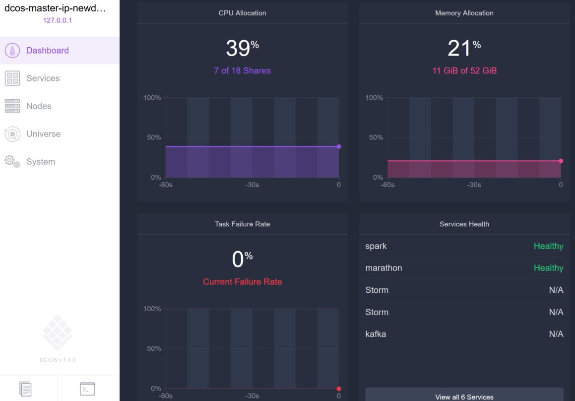Figure 1. DCOS web interface.

DCOS is the distributed cluster operating system and its job is to support deployed services. The most valuable of these services is Marathon which is a container orchestration service that will allow you to easily scale the number instances of your containers and keep them running. It can also be used to enforce special constraints. For example, if you deploy a docker container that needs to bind to a special port on they host, it will not schedule another conflicting instance on that same host. And it has a very nice graphical user interface shown in figure 2 that can be accessed through the DCOS interface.

Figure 2. Marathon interface showing all running services.

As you can see above I have an instance of Apache Spark, two instances of the streaming service Storm and one instance of the Zeppelin notebook and one instance of the simple web server Nginx all running. Launching a new Docker container or service is very simple: fill in a web-form. However, there is a command line tool that works very well on linux and windows. For example, to get the information in Figure 2 above the command line call is as follows.

The same command line interface can be used to launch new container instances and we will illustrate that below.

DCOS also has views of the of the individual resources. Figure 3 displays the current view of all of the individual nodes in the cluster showing how many of the nodes are holding active containers or services.

Figure 3. DCOS display of worker node status and load

A Simple Example.

There are many prepackaged apps available for a one-click launch such as those listed above. I originally wanted to Kafka in a demo, but there is still a bug with my deployment that does not allow me to access the Kafka gateway or the public node (10.0.0.5 in the Figure 3 list). I will revise this report with an update as soon as I can solve that problem.

The example is a simple message filtering experiment. Assume you have some source of independent tasks that must be analyzed as fast as possible and the results stored in a table or database. Assume further that you task stream can be pre-filtered into and sorted into buckets of similar tasks that can be analyzed by code that is best suited for the tasks in that bucket. For example, some tasks contain images of landscapes and others contain images of animals and you want to provide analyzers that are appropriate for each. Or you are looking at logging data and your pre-filters detect several different types of anomalies and you want to group anomalies of similar type together. We will use queues to hold the contents of each bucket. The pre-filters push the data into the queues and workers pull the tasks of the queue, do the analysis and push the results to into a table. The general picture is shown in Figure 4 below.

Figure 4. Sample “microservice” configuration for our experiment.

Depending upon the complexity of the analysis undertaken by the worker and the arrival rate of tasks into the queues we may need to increase the number of workers assigned to each bucket queue as shown in Figure 5.

Figure 5. Adding additional workers to manage extra work at each queue.

In this simple experiment we will look at how increasing the number of workers can improve the throughput of the system. Now for the details of the set-up. Instead of using Kafka, we will use another common message broker RabbitMQ that is running on another linux box on Azure. We use the Azure Table service to store the results. Our worker service is a Docker container that is running a simple Python program that has two parts.

When the worker starts-up it does not know what queue to list to. So it looks in a separate queue called “roles” that will contain the name of the queue needed an extra worker.
When it has the name of the queue to work on and begin pulling data items from the given queue and processing them and saving them to the table. A time stamp is added to each item as it goes into the table.

In a real application step 2 can include task specialization once the worker knows what queue it is working on. For example, in our text classifier example we loaded specific machine learning tables and states when we knew what topics we were analyzing.

In this example, we are only interested in the basic scale-up performance improvement as we increase the number of workers assigned to each queue. The Python code for the container is not pretty, but you are welcome to read and use it. It is on GitHub here. To deploy the Docker container on DCOS one needs a deployment configuration json file. This config.json is shown below.

{
   "container": {
      "type": "DOCKER",
      "docker": {
          "image": "escigrp/rabbitpullpush"
       }
    },
   "id": "worker",
   "instances": 1,
   "cpus": 0.2,
   "mem": 512,
}

Notice that this specifies that the container is in the Docker hub with the name escigrp/rabbitpullpush and that we wish to devote 0.2 cpus and 512 MB of memory to this resource. And we want one instance.

The dcos command to launch this container in the cluster is

dcos marathon app add config.json

Our “worker” will immediately show up as a deployment on the DCOS Marathon web page.

We are going to measure the throughput of the system in the number of events per second it can process as we increase the number of workers per node. The way the experiment is done is as follows

For N = 1 to 14:

Preload each of the 4 queues (named “1”, “2”, “3”, “4”) with 500 messages and start up 4*N instances of the worker container with Marathon on DCOS.
Load the “roles” queue with N instances of each queue name. Each of the four queues will now have N devoted workers.
When all of the queues are empty, look in the table. Subtract the earliest time stamp from the latest to get an approximation of the elapsed time.
Use marathon to shutdown the workers and go to step 1.

Recall that there are 8 dual core nodes in the cluster. Each instance of the worker container is allocated 0.2 of a core. This means marathon could possibly schedule 80 instances. However, there are other processes running on cluster so a practical limit was 60. In fact we tested up to 56 container instances (14*4). The results are shown in Figure 6 below.

Figure 6. Events processed per second as the number of workers per queue grows from 1 to 14.

There are several surprises for me here. First the performance scales very linearly as the number of container instances grows. Because there are only 16 cores available I expected this to level off when N was near 8 (32 instances), but, with the exception of an anomaly around 13, it kept climbing to N = 14 (56 instances). Second, the absolute performance is not very good. Digging deeper into the code and conducting several additional experiments revealed that the bottleneck is the table insertion due to an old and slow version of the python library. Without the table insertion a single worker container instance call pull events at a rate of about 20 events per second, so 56 instances will be over 1000 events/sec which is well within the range of RabbitMQ.

Dynamic Scaling and Conclusion

A more interesting experiment would be to have the system described above dynamically scale the number of container instances as circumstances require. For example, if one could monitor the depth of each queue, then if a queue starts to grow larger one could issue a command to increase the number of instances devoted to that queue. If the queue is empty one could reduce the number of instances. I am fairly certain there are a number of ways to do this, but one easy way is to use the “marathon update” command. This command allows a “real-time” update to json configuration. Any field in the configuration can be modified. For example, to update the configuration to 10 instances one can issue the command below.

dcos marathon app update worker env='{"instances":"10"}'

This change in status should trigger marathon to make the necessary adjustments and change the number of instances to 10. It would be relatively straight forward to write a program that would poll the event broker for status and check the current queue lengths and, depending on the conditions issue the dcos command above.

Final Thoughts.

It is great to see this container service based on Mesosphere’s DC/OS finally available in a reliable and highly usable form. This an excellent platform for managing large collections of Docker containers and orchestrating microservices deployments. The performance of the system was excellent and the web user interface is well done. The command line interface is solid and only gave me one problem. Installing the command line interface for Kafka caused problems on windows and it did not follow the script here. It seemed to be loading an old version that did not support windows. The other problem was that the DC/OS cluster I deployed on Azure had one public node, but the “public” IP address give for this node was not reachable. (Any reader who knows how to address these problems please comment here and I will update this post. As is often the case, there are easy solutions to problems that stump me.)

In a future post we will look at the Docker Swarm deployment that is also part of this new Azure release.

Fun with Recurrent Neural Nets: One More Dive into CNTK and TensorFlow

In a previous article I set about comparing Microsoft’s Computational Network Took Kit for deep neural nets to Google’s TensorFlow. I concluded that piece with a deep dive into how recurrent neural nets (RNNs) were represented in each system. I specifically went after the type of RNNs known by the strange name of Long Short-Term Memory (LSTM) networks. I wanted to learn a bit more about how these systems worked. I decided to treat them like laboratory specimens so that I could poke and prod them to see what I could learn and what I could get them to do. This article is essentially my lab notebook. Warning: With the exception of a bit toward the end, this is not technically very deep. In fact, I did not discover anything that has not been extensively reported on elsewhere. But I learned a lot and had some fun. Perhaps it will be of interest to students just starting to learn about this subject. Before I get to far into this, I would like to mention that I recently discovered an excellent series of tutorials on RNNs by Denny Britz that are definitely worth reading.

CNTK’s LSTM and Hallucinating Bloomberg Financial News

One of the many good examples in CNTK is language modeling exercise in Examples/Text/PennTreebank. The documentation for this one is a bit sparse and the example is really just of a demo for how easy it is to use their “Simple Network Builder” to define a LSTM network and train it with stochastic gradient decent on data from the Penn Treebank Project. One command starts the learning:

cntk configFile=../Config/rnn.cntk

Doing so trains the network, tests it and saves the model. However, to see the model data in an easily readable form you need a trivial addition to the configfile: you need to add the following dumpnode command to put a dump file a directory of your choosing.

dumpnode=[
    action = "dumpnode"
    modelPath = "$ModelDir$/rnn.dnn"
    outputFile = "$OutputDir$/modeltext/dump"
]

This creates a big text file with all the trained data. To experiment with the trained model, I decided to load it into a python notebook and rebuild the LSTM network from the defining equations. From the CNTK book those equations are

I was pleased to see that the dumped model text had the same W and b tensors names as in the equations, so my job was relatively easy. I extracted each of the tensors and saved them into a file (I will make these available in Github). The python code for the LSTM based on the equations above is below.

def rnn(word, old_h, old_c):
      Xvec = getvec(word, E)

      i = Sigmoid(np.matmul(WXI, Xvec) + 
                  np.matmul(WHI, old_h) + WCI*old_c + bI)
      f = Sigmoid(np.matmul(WXF, Xvec) + 
                  np.matmul(WHF, old_h) + WCF*old_c + bF)
      
      c = f*old_c + i*(np.tanh(np.matmul(WXC, Xvec) + 
                               np.matmul(WHC, old_h) + bC))
      
      o = Sigmoid(np.matmul(WXO, Xvec)+ 
                  np.matmul(WHO, old_h)+ (WCO * c)+ bO)
      
      h = o * np.tanh(c)
      
      #extract ordered list of five best possible next words
      q = h.copy()
      q.shape = (1, 200)
      output = np.matmul(q, W2)
      outlist = getwordsfromoutput(output)
      return h, c, outlist

As you can see, this is almost a literal translation of the equations. The only different is that this has as input a text string for the input word. However the input to the equations is a vector encoding of the word. The model generates the encoding matrix E which has the nice property that the i^th column of matrix corresponds to the word in the i^th position in the vocabulary list. The function getvec(word, E) takes the embedding tensor E, and looks up the position of the word in the vocabulary list and returns the column vector of E that corresponds to that word. The output of one pass through the LSTM cell is the vector h. This is a compact representation of the words likely to follow the input text to this point. To convert this back into “vocabulary” space we multiply it by another trained vector W2. The size of our vocabulary is 10000 and the vector output is that length. The i^th element of output represents the relative likelihood that that i^th word is next word to follow the input so far. Getwordsfromoutput simply returns the top 5 candidate words in order of likelihood.

Before going further, it is worth looking closer at the properties of the word embedding matrices E and W2. There is a fascinating paper by Mikolov, Yih and Zweig entitled “Linguistic Regularities in Continuous Space Word Representations” where they suggest that the embedding space for word has several interesting properties. I decided to investigate that. Their point is that words that are similar in a linguistic sense will be nearby in the embedding space. For example, present tense verbs should be near other present tense verbs and singular nouns should be near each other, etc. I decided to try that. However, there are two embedding mappings. One is based on the tensor E and the other based on the W2 tensor. E has dimension 150 by 10000 and W2 is 200 by 10000. The difference in dimensionality are because of arbitrary decisions made in defining the hidden layers in the network. But both represent word imbeddings. I experimented with both. I wrote a function getnear(word, M) which takes a word and looks for the 5 most nearby words in the space where M is transpose of either E or W2. (I used cosine distance as the metric.) Verb tense locality and noun plurals worked best in the W2 space as illustrated below.

These are only illustrations. For a deeper statistical analysis look at the Mikolov paper. A more interesting conjecture from their study was that there may be some linearity in these embedding that might allow one to try simple analogies of the form “A is to B, as C is to __”. Their idea is that if a, b and c are the vector embeddings of the words A, B and C, then the embedding of “__” may be computed as d = c + (b-a). So I wrote a little function AistoBasCisto(A, B, C) that does this computation. In the results I had to delete A, B and C from the candidate answers because they came up often as nearby. In this case my results were less encouraging. It worked better with the E space than with W2. For example, for E we have

And for the W2 space the results looked like

As you can see the “run running walk __” example failed with E but was close, but still incorrect, with W2.

You may wonder why these particular words came up. The data we used to train the system came from a small subset of the Penn TreeBank collection as provided in the CNTK package. It is heavily dominated by financial news items. This explains why the plural of person could be managers or customers. A larger vocabulary and data collection would be needed to truly test the analogy by linearity conjecture.

Now on to hallucinating the financial news.

Now to test the LSTM as a truly recurrent network. We provide the network with a starting word and let it suggest the next word. And then we repeat this process constructing a “sentence”. In the code below we randomly pick one of the top three suggest by the network as the next word.

c = np.zeros(shape = (200, 1))
h = np.zeros(shape = (200, 1))
output = np.zeros(shape = (10000, 1))
word = 'my'
sentence= word 
for _ in range(40):
    h, c, outlist = rnn(word, h, c)
    word = outlist[randint(0,3)]
    sentence = sentence + " " +word
print sentence+"."

In this case we start with the word “my” and let it generate a 40 word sentence. The output is

my new rules which would create an interest position here unless there should prove   signs of such things too quickly although the market could be done better toward paying further volatility where it would pay cash around again if everybody can.

This is a great example of hallucinating financial news. Let’s try it again starting with the word “president”.

president michael de brown wrote himself against democratic union law which represents an emergency relief agreement during a new york state district or early tuesday before july after a federal government agency created early losses without mr. krenz or perhaps.

Now with the word “the”.

the company reported third-quarter results reflecting a number compared between N barrels including pretax operating loss from a month following fiscal month ending july earlier compared slightly higher while six-month cds increased sharply tuesday after an after-tax loss reflecting a strong.

The “sentences” end rather abruptly because of the 40 word limit I set. If you let it go it will run on until the state vector for the sentence seems to break down. Try this yourself. To make it easy to play with this example, I have put the code in GitHub. The trained model text files are in OneDrive and is a zipped file of about 50MB.

There are many more excellent and fun examples. Andrej Karpathy has a great blog article showing how RNNs can mimic Shakespeare, or Latex science articles and many more.

TensorFlow’s seq2seq French Lesson.

One of the most interesting examples in the TensorFlow tutorials is an English to French translator. As with the CNTK example it was trivial to start the translator learning following the instructions in the tutorial. After letting this run for about a week, I wanted to see how well it would do. As with the CNTK example, I created a Jupyter IPython notebook and loaded the trained model. I will explain how that was done in more detail below but, for now, I will show how we can invoke it to test its translation ability. This particular trained model was not very big and with a relatively small data set, so I didn’t expect much. In fact, as you will see, to a French speaker it is a disaster. On the other hand, it learned more French in a week of training that I did in three semesters of French in college. (For full disclosure, this was my weakest subject in college and my grade was a hard-fought “C” each semester.)

The code below demonstrates how the model is invoked. First you have to tokenize the input sentence. The algorithm uses a system of buckets of fixed sizes to make the training more efficient. You next find the smallest bucket that can contain your sentence and convert this to the input vector list needed by the model. The step function takes a Tensorflow session, the input vector list and a null list of decoder inputs (to be explained later) and generates a list of vectors as outputs. Each vector represents the likelihood that individual vocabulary words are the correct word at that point in the translated sentence. We pick the most likely and print the sentence.

sentence = " I am not the president of France. "

token_ids = data_utils.sentence_to_token_ids(sentence, en_vocab)
      # Which bucket does it belong to?
bucket_id = min([b for b in xrange(len(_buckets))
                 if _buckets[b][0] > len(token_ids)])
      # Get a 1-element batch to feed the sentence to the model.
encoder_inputs, decoder_inputs, target_weights = 
    model.get_batch({bucket_id: [(token_ids, [])]}, bucket_id)

_, _, output_logits = model.step(sess, encoder_inputs, decoder_inputs, 
                                 target_weights, bucket_id, True)
		  
outputs = [int(np.argmax(logit, axis=1)) for logit in output_logits]
print(" ".join([rev_fr_vocab[output] for output in outputs]))

Je ne suis pas le président de la France .

This example is not too bad. However, if I ask

“In which city does the president of France live?”

I get

“Dans quelle ville le président de la France ?”.

This is not exactly correct. If I feed this into Google translate and ask what this means in English I get “In which city the President of France?”. If I give it this one,

” What is the name of a good restaurant? ”

The system responds with

“Quel est le nom d’une bonne bonne bonne ?”

Which translates back to “What is the name of a good good good?”. Probably not very helpful on the streets of Paris. It turns out restaurant is not in the tiny training vocabulary used here. Finally, given this sentence

” The article stated that the President of the United States is here today. “

The translator returned

“Le paragraphe a indiqué que le président des États-Unis est aujourd ‘ hui aujourd ‘ hui .”

The end of this reply is “is today today”. As I said, this is still much better than I could do with my college French. However, as you can see from the previous two examples, our little translator runs out of gas at the end of sentences and tends to repeat itself. You should try this yourself. I have put the notebook file in github or you can execute these directly from the Tensorflow python code. All you need to do is train the model from TensorFlow and run the notebook with the path to the model output directory.

While loading and using the trained model was easy and fun, understanding the seq2seq model used in this example takes a bit of work. So this part of this article will get a bit more technical.

The TensorFlow translate program is based on a sequence-to-sequence model constructed from more primitive recurrent neural nets. By sequence-to-sequence we mean a network that takes a sequence as input and produces a sequence as output. It consists of two parts: an “encoder RNN” and a “decoder RNN” as shown in Figure 1 below.

Figure 1. A sequence-to-sequence RNN English to French translator with the encoder and decoder unrolled to show the flow of messages.

In this figure the RNNs are “unrolled” to show the flow of messages. The state vector at the end of the encoder is a vector embedding of the input sentence. This state vector is used to start the decoder along with a “GO” token. The diagram shows the network after it has been trained. During training the inputs to the decoder are the French version of the English sentences. I won’t talk about the training here because is enough to try to understand how this works. Before I go any further I want to point you to some important papers. Sutskever, Vinyals and Le published an early important paper on sequence to sequence models that is worth reading.

To understand how it is built the network we need to dig into the code a bit. The building blocks are a set of classes of base type RNNCell with specializations

BasicRNNCell
GRUCell
BasicLSTMCell
LSTMCell
OutputProjectionWrapper
InputProjectionWrapper
EmbeddingWrapper
MultiRNNCell

The ones we will see used here are GRUCell, MultiRNNCell and EmbeddingWrapper. We discussed LSTMCell in our previous article but we need to look at GRUCell here because that is the one used in the example. The GRUCell is a “Gated Recurrent Unit” invented by Cho et. al. in “Learning Phrase Representations using RNN Encoder–Decoder for Statistical Machine Translation”. The “gated” phrase comes from the way the output is defined as coming mostly from the previous state or from a combination with the new input. The diagram below tries to explain this a bit better.

Figure 2. GRU wiring diagram

It also helps to see it in terms of the defining equations.

The quantity u_t is a gate vector. Recall the sigmoid function switches sharply between one and zero. So when u_tis one then h is just a copy of the old h and we are ignoring the input x it is based on the value c_t. The gate r_t is determines how much of the old state goes into defining the value of c_t. To understand how this is encoded in TensorFlow you need to understand the function.

linear(args, output_size, bias, bias_start=0.0, scope=None)

where args is a list of tensors each of size batch x n . Linear computes sum_i(args[i] * W[i]) + bias where W is a list of matrix variables of size n x outputsize and bias is a variable of size outputsize. In the equations above we have represented linear algebra as a matrix times a column vector. Tensorflow uses the transpose notation: row vector on the left times the transpose of the matrix. So in linear the args are a list of row vectors. Where is the matrix W and offset b? This is fetched from memory based on the variable current scope, because W and b are variable tensors that are learned values. If you look at the first two equations above, you will see they are almost identical. In fact, we can write them as

If you transpose the last one from column form into row form you can now compute both with one invocation of the linear function. The code for the GRUCell is below. As you can see they have encoded one pass through the GRU cell with only two matrix vector multiplies. You can also see that the way the variable scope is used to pick out the W’s for the gates and the W for the state/output. Another point to remember that an invocation of the “__call__ function operator does not cause the tensor to execute the operation, rather it builds the graph.

class GRUCell(RNNCell):
  def __init__(self, num_units):
    self._num_units = num_units
   ... stuff deleted ....
  def __call__(self, inputs, state, scope=None):
    with vs.variable_scope(scope or type(self).__name__):  
      with vs.variable_scope("Gates"):  # Reset gate and update gate.
        # We start with bias of 1.0 to not reset and not udpate.
        r, u = array_ops.split(1, 2, linear([inputs, state],  
                               2 * self._num_units, True, 1.0))
        r, u = sigmoid(r), sigmoid(u)
      with vs.variable_scope("Candidate"):
        c = tanh(linear([inputs, r * state], self._num_units, True))
      new_h = u * state + (1 - u) * c
    return new_h, new_h

The top level class we invoke for building our model is seq2seqModel. When we create an instance of this class it sets in motion a set of flowgraph building steps. I am going to skip over a lot of stuff and try to give you the big picture. The first graph building step in the initialization of an instance of this object is

# Create the internal multi-layer cell for our RNN.
    single_cell = rnn_cell.GRUCell(size)
     …
    if num_layers > 1:
      cell = rnn_cell.MultiRNNCell([single_cell] * num_layers)

As you can see we are creating a GRU cell graph generator instance and making a list of num_layers of this object and passing that to the constructor for MultiRNNCell. In our case, num_layers has been set to 2. MultiRNNCell is pretty easy to understand. It builds a graph consisting of a stack of (in this case) GRU cells where the output state vector of each level is fed to the input of the level above it. This new compound cell has an output that is the state of the top sub-cell and whose output state is the concatenation of the output states of all the sub-cells.

The next part is not so easy to follow. We will take our MultiRNNCell graph builder and use it to create and encoder and a special decoder. But first we must make a short digression.

Paying Attention

There is a problem that is encountered in the sequence-to-sequence model. The encoder encodes the entire sentence into a state vector which is used by the decoder as its input. That state vector is an abstract representation of our entire sentence as a single point in a very high dimensional space. The decoder has been trained to use that point as a starting point to unroll a translated version of the sentence. I find the fact that it works at all to be rather remarkable. It is as if the decoder takes the English state vector and transforms it into a similar point in “French” space.

Unfortunately, the longer the input sentence, the more difficult it is to decode it. How much information can we pack into one point? The problem is that at each decoding step we need a little bit more information than is provided by the state vector as it passes through the decoder loop. The idea used here is to help the decoder by providing it a bit of focus derived from the input sequence at each stage of the decoder loop. This is generally referred to as “attention”, as in “at this step of decoding please pay attention to what the encoder was doing here”. Bahdanau, Cho and Bengio had an early paper about this that used a bidirectional pass over the input sequence. As they put it, they wanted to “automatically (soft-)search for parts of a source sentence that are relevant to predicting a target word”. (Denny Britz has a lovely blog article about attention and describes several fascinating applications. It is well worth reading.) The mechanism for attention used in the TensorFlow example is based on a paper by Vinyals et. al. and we will follow that one here. The key idea is rather than take the single final state vector from the encoder, let’s collect the state vectors at each stage of the encoder. Following Vinyals, let the encoder state vectors for each input word be

And let the decoder state vectors be

Then for each decoder time step t compute

Where the Ws are learned matrices and v is a learned vector. Then as the input to the t+1 state vector of the decoder we use the concatenation

The idea is this new state vector at time t+1 puts much more focus on the corresponding words in in the encoder string. This all happens in a function called seq2seq.attention_decoder that is called in another constructor function seq2seq.embedding_attention_seq2seq that wraps and an embedding around a graph generated by our MultiCellRNN graph builder to generate the final decoder graph. These graphs are all stitched together in the Seq2SeqModel constructor. It is fair to say that there are many levels of abstraction here that are used to build the decoder and link it to the encoder. I am leaving out many details that are critical for the training such as the part that implements the bucket handler. The final graph, in its most abstract form is pictured below in figure 3.

Figure 3. The Translate.py sequence to sequence translator is based on a two level GRU cell encoder and an attention-augmented two level GRU cell decoder. The input English is entered in reverse order as an optimization

Final Thoughts

As I have said above, I have not included all the details of how the seq2seq translator is put together, but I tried to include the highlights that I found most interesting. I encourage you to dive into the code and discover the rest. You will likely find some errors in what I described above. If so, please let me know.

There is really a lot of exciting results that have come out in the last few years relating to RNNs. For example, Lei Ba, Mnih and Kavukcuoglu demonstrated that RNNs with attention can be applied to interesting image analysis challenges, such as reading the house number from a street scene. In “Teaching Machines to Read and Comprehend” Hermann et. al. excellent paper demonstrate the use of an attentive RNN build to answer simple questions about text. I personally don’t think any RNN can pass a Turing test yet, so it ain’t A.I. But these little statistical machines are certainly wonderful mimics and they can speak better French than I.