
In July 2021 Alex Davies and a team from DeepMind, Oxford and University of Sydney published a paper entitled “Advancing mathematics by guiding human intuition with AI”. The paper addresses the question of how can machine learning be used to guide intuition in mathematical discovery? The formal approach they take to this question proceeds as follows. Let Z be a collection of objects. Suppose that for each instance z in Z we have two distinct mathematical representations of z: X(z) and Y(z). We can then ask, without knowing z, is there a mathematical function f : X -> Y such that given X(z) and Y(z), f(X(z)) = Y(z)? Suppose the mathematician builds a machine learning model trained on many instances of X(z) and Y(z). That model can be thought of as a function f^ :X -> Y such that f^(X(z)) ~ Y(z). The question then becomes, can we use properties of that model to give us clues on how to construct the true f?
A really simple example that the authors give is to let Z be the set of convex polyhedral (cube, tetrahedron, octahedron, etc.). If we let X(z) be the tuple of numbers defined by the number of edges, the number of vertices, the volume of z and the surface area and let Y(z) be the number of faces, then without knowing z, the question becomes is there a function f: R4 -> R such that f( X(z) ) = Y(z) ? Euler answered this question some time ago in the affirmative: Yes, he proved that
f(edges, vertices, volume, surface area) = edges – vertices + 2 = faces.
Now suppose we did not have Euler to help us. Given a big table where each row corresponds to (edge, vertices, volume, surface area, faces) for some convex polytope, we can select a subset of rows as a training set and try to build a model to predict faces given the other values. Should our AI model prove highly accurate on the test set consisting of the unselected rows, that may lead us to suspect that such a function exists. In a statistical sense, the learned model is such a function, but it may not be exact and, worse, by itself, it may not lead us to formula as satisfying as Euler’s.
This leads us to Explainable AI. This is a topic that has grown in importance over the last decade as machine learning has been making more and more decisions “on our behalf”. Such as which movies we should rent and which social media article we should read. We wonder “Why did the recommender come to the conclusion that I would like that movie?” This is now a big area of research (the Wikipedia article has a substantial bibliography on Explainable AI.) One outcome of this work has been a set of methods that can be applied to trained models to help us understand what parts of the data are most critical in the model’s decision making. Davies and his team are interested in understanding what are the most “salient” features of X(z) in relation to determining Y(z) and using this knowledge to inspire the mathematician’s intuition in the search for f. We return to their mathematical examples later, but first let’s look closer at the concept of salience.
Salience and Integrated Gradients
Our goal is to understand how important each feature of the input to a neural network is to the outcome. The features that are most important are often referred to as “salient” features. In a very nice paper, Axiomatic Attribution for Deep Networks from 2017 Sundararajan, Taly and Yan consider this the question of attribution. When considering the attribution of input features to output results of DNNs, they propose two reasonable axioms. The first is Sensitivity: if a feature of the input causes the network to make a change then that feature should have a non-zero attribution. In other words, it is salient. Represent the network as a function F: Rn->[0,1] for n-dimensional data. In order to make the discussion more precise we need to pick a baseline input x’ that represents the network in an inactivated state: F(x’) = 0. For example, in a vision system, an image that is all black will do. We are interested in finding the features in x that are critical when F(x) is near 1.
The second axiom is more subtle. Implementation Invariance: If two neural networks are equivalent (i.e. they give the same results for the same input), the attribution of a feature should be the same for both.
The simples form of salience computation is to look at the gradient of the network. For each i in 1 .. n, we can look at the components of the gradient and define

This axiom satisfies implementation invariance, but unfortunately this fails the sensitivity test. The problem is the value of F(xe) for some xe may be 1, but the gradient may be 0 at that point. We will show an example of this below. On the other hand if we think about “increasing” x from x’ to xe , there should be a transition of the gradient from 0 to non-zero as F(x) increases towards 1. That motivates the definition of Integrated Gradients. We are going to add up the values of the gradient along a path from the baseline to a value that causes the network to change.
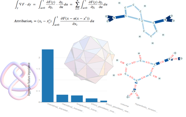
let γ = (γ1, . . . , γn) : [0, 1] → Rn be a smooth function specifying a path in Rn from the baseline x’ to the input x, i.e., γ(0) = x’ and γ(1) = x. It turns out that it doesn’t matter which path we take because we will be approximating the path integral, and by the fundamental theorem of calculus applied to path integrals, we have

Expanding the integral out in terms of the components of the gradient,

Now, picking the path that represents the straight line between x’ and x as

Substituting this in the right-hand side and simplifying, we can set the attribution for the ith component as

To compute the attribution of factor i, for input x, we need only evaluate the gradient along the path at several points to approximate the integral. In the examples below we show how salience in this form and others may be used to give us some knowledge about our understanding problem.
Digression: Computing Salience and Integrated Gradients using Torch
Readers not interested in how to do the computation of salience in PyTorch can skip this section and go on to the next section on Mathematical Intuition and Knots.
A team from Facebook AI introduced Captum in 2019 as a library designed to compute many types of salience models. It is designed to work with PyTorch deep learning tools. To illustrate it we will look at a simple example to show where simple gradient salience breaks down yet integrated gradience works fine. The complete details of this example are in this notebook on Github.
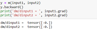
We start with the following really dumb neural network consisting of one relu operator on two input parameters.

A quick look at this suggests that the most salient parameter is input1 (because it has 10 time the influence on the result of input2. Of course, the relu operator tells us that result is flat for large positive values of input1 and input2. We see that as follows.


We can directly compute the gradient using basic automatic differentiation in Torch. When we evaluate the partial derivatives for these values of input1 and input2 we see they are zero.
From Captum we can grab the IntegratedGradient and Salience operators and apply them as follows.

The integrated Gradient approximation shows that indeed input1 has 10 time the attribution strength of input2. And the sum of these is m(input1, input2) plus an error term. As we already expect, the simple gradient method of computing salience will fail.

Of course this extreme example does not mean simple gradient salience will fail all the time. We will return to Captum (but without the details) in another example later in this article.
Mathematical Intuition and Knots
Returning to mathematics, the Davies team considered two problems. The methodology they used is described in the figure below which roughly corresponds to our discussion in the introduction.

Figure 1. Experimental methodology used by Davies, et.al. (Figure 1 from “Advancing mathematics by guiding human intuition with AI”. Nature, Vol 600, 2 December 2021)
They began with a conjecture about Knot theory. Specifically, they were interested in the conjecture that that the geometric invariants of knots (playing the role of X(z) in the scenario above) could determine some of the algebraic invariants (as Y(z)). See Figure 2 below.

Figure 2. Geometric and algebraic invariant of hyperbolic knots. (Figure 2 from “Advancing mathematics by guiding human intuition with AI”. Nature, Vol 600, 2 December 2021)
The authors of the paper had access to information 18 geometric invariants on 243,000 knots and built a custom deep learning stack to try to identify the salient invariants that could identify the signature of the knot (a snapshot of the information is shown below). Rather than describing their model, we decided to apply one generated by the AutoML tool provided by the Azure ML Studio.

Figure 3. Snapshot of the Knot invariant data rendered as a python pandas dataframe.
We uses a Jupyter Notebook to interact with the remote instances of the azure ML studio. The notebook is in github here: dbgannon/math: Notebooks from Explainable Deep Learning and Guiding Human Intuition with AI (github.com). The notebook also contains links to the dataset.
Because we described azure ML studio in a previous post, we will not go into it here in detail. We formulated the computation as a straightforward regression classification problem. AutoML completed the model selection and training and it also computed the factor salience computation with the results shown below.

Figure 4. Salience of features computed by Azure AutoML using their Machine Learning services (To see the salience factors one has to look at the output details on the ML studio page for the computation.)
The three top factors were: the real and imaginary components of meridinal_translation, and the longitudinal translation. These are the same top factors that were revealed in the authors study but in a different order.
Based on this hint they authors proposed a conjecture: for a hyperbolic knot K define the slope(K) to be the real part of the fraction longitudinal translation/meridinal_translation. Then there exists constants c1 and c2 such that

In Figure 5, we show scatter plots of the predicted signature versus the real signature of each of the knots in the test suit. As you can see, the predicted signatures form a reasonably tight band around the diagonal (true signatures). The mean squared error of the formula slope(K)/2 from the true signature was 0.86 and the mean squared error of the model predictions was 0.37. This suggests that the conjecture may need some small correction terms, but that is up to the mathematician to prove. Otherwise, we suspect the bounds in the inequality are reasonable.

Figure 5. On the left is a scatter plot of the slope(K)/2 computed from the geometric data vs the signature. On the right is the signature predicted by the model vs the signature.
Graph Neural Nets and Salient Subgraphs.
The second problem that the team looked at involved representation theory. In this case they are interested in pairs of elements in the symmetric group Sn represented as permutations. For example, in S5 an instance z might be {(03214), (34201)}. An interesting question to study is how to transform the first permutation into the second by simple 2-element exchanges (rotations) such as 03214->13204->31204->34201. In fact, there are many ways to do this and we can build a directed graph showing the various paths of rotations to get from the first to the second. This graph is called the unlabeled Bruhat interval, and it is their X(z). The Y(z) is the Kazhdan–Lusztig (KL) polynomial for the permutation pair. To go any deeper into this topic is way beyond the scope of this article (and beyond the knowledge of this author!) Rather, we shall jump to their conclusion and then consider a different problem related to salient subgraphs. They discovered by looking at salient subgraphs of a Bruhat interval graph a for a pair in Sn that there was a hypercube and a subgraph isomorphic to an interval in Sn−1. This led to a formula for computing the KL polynomial. A very hard problem solved!
An important observation the authors used in designing the neural net model was that information conveyed along the Bruhat interval was similar to message passing models in Graph neural networks. These GNNs have become powerful tools for many problems. We will use a different example to illustrate the use of salience in understanding graph structures. The example is one of the demo cases for the excellent Pytorch Geometric libraries. More specifically it is one of their example Colab Notebooks and Video Tutorials — pytorch_geometric 2.0.4 documentation (pytorch-geometric.readthedocs.io). The example illustrates the use of graph neural networks for classification of molecular structures for use as drug candidates.
Mutagenicity is a property of a chemical compound that hampers its potential to become a safe drug. Specifically there are often substructures of a compound, called toxicophores, that can interact with proteins or DNA that can lead to changes in the normal cellular biochemistry. An article from J. Med. Chem. 2005, 48, 1, 312–320, describes a collection of 4337 (2401 mutagens and 1936 nonmutagens). These are included in the TUDataset collection and used here.
The Pytorch Geometric example uses the Captum library (that we illustrated above) to identify the salient substructures that are likely toxicophores. While we will not go into great detail about the notebook because it is in their Colab space. If you want to run this on your on machine we have put a copy in our github folder for this project.
The TUDataset data set encodes molecules, such as the graph below, as an object of the form
Data( edge_index=[2, 26], x=[13, 14], y=[1] )

In this object x represents the 13 vertices (atoms). There are 14 properties associated with each atom, but they are just ‘one-hot’ encodings of the names of each of the 14 possible elements in the dataset: ‘C’, ‘O’, ‘Cl’, ‘H’, ‘N’, ‘F’,’Br’, ‘S’, ‘P’, ‘I’, ‘Na’, ‘K’, ‘Li’, ‘Ca’. The edge index represents the 26 edges where each is identified by the index of the 2 end atoms. The value Y is 0 if this molecule is known to be mutagenic and 1 otherwise.
We must first train a graph neural network that will learn to recognize the mutagenic molecules. Once we have that trained network, we can apply Captum’s IntegratedGradient to identify the salient subgraphs that most implicate the whole graph as mutagenic.
The neural network is a five layer graph convolutional network. A convolutional graph layer works by adding together information from each graph neighbor of each node and multiplying it by a trainable matrix. More specifically assume that each node has a vector xl of values at level l. We then compute a new vector xl+1 of values for node v at level l+1 by

where 𝐖(ℓ+1) denotes a trainable weight matrix of shape [num_outputs, num_inputs] and 𝑐𝑤,𝑣 refers to a fixed normalization coefficient for each edge. In our case 𝑐𝑤,𝑣 is the number of edges coming into node v divided by the weight of the edge. Our network is described below.

The forward method uses the x node property and the edge index map to guide the convolutional steps. Note that we will use batches of molecules in the training and the parameter batch is how we can distinguish one molecule from another, so that the vector x is finally a pair of values for each element of the batch. With edge_weight set to None, the weight of each edge is a constant 1.0.
The training step is a totally standard PyTorch training loop. With the dim variable set to 64 and 200 epochs later, the training accuracy is 96% and test accuracy is 84%. To compute the salient subgraphs using integrated gradients we will have to compute the partial derivate of the model with respect to each of the edge weights. To do so, we replace the edge weight with a variable tensor whose value is 1.0.
Looking at a sample from the set of mutagenic molecules, we can view the integrated gradients for each edge. In figure 6 below on the left we show a sample with the edges labeled by their IG values. To make this easier to see the example code replaces the IG values with a color code where large IG values have thicker darker lines.
The article from J. Med. Chem notes that the occurrence of NO2 is often a sign of mutagenicity, so we are not surprised to see it in this example. In Figure 7, we show several other examples that illustrate different salient subgraphs.

Figure 6. The sample from the Mutagenic set with the IngetratedGradient values labeling the edges. On the right we have a version with dark, heavy lines representing large IG values.

Figure 7. Four more samples. The subgraph N02 in the upper left is clearly salient, but in the three other examples we see COH bonds showing salient subgraphs. However these also occur in the other, non-mutagenic set, so the significance is not clear to us non-experts.
Conclusion.
The issue of explainability of ML methods is clearly important when we let ML make decisions about peoples lives. Salience analysis lies at the heart of the contribution to mathematical insight described above. We have attempted to illustrate where it can be used to help us learn about the features in training data that drive classification systems to draw conclusions. However, it takes the inspiration of a human expert to understand how those features are fundamentally related to the outcome.
ML methods are having a far-reaching impact throughout scientific endeavors. Deep learning has become a new tool that is used in research in particle physics to improve the search for signals in data, in astronomy where generative methods can create galaxy models for dark energy experiments and biochemistry where RoseTTAFold and DeepMind’s AlphaFold have used deep learning models to revolutionize protein folding and protein-protein interaction. The models constructed in these cases are composed from well-understood components such as GANs and Transformers where issues of explainability have more to do with optimization of the model and its resources usage. We will return to that topic in a future study.
