Edge computing describes the movement of computation away from cloud data centers so that it can be closer to instruments, sensors and actuators where it will be run on “small” embedded computers or nearby “micro-datacenters”.  The primary reason to do this is to avoid the network latency in cases where responding to a local event is time critical.  This is clearly the case for robots such as autonomous vehicles, but it is also true of controlling many scientific or industrial apparatuses.  In other cases, privacy concerns can prohibit sending the data over an external network.

We have now entered the age where advances in machine learning has made it possible to infer much more knowledge from a collection of the sensors than was possible a decade ago.    The question we address here is how much deep computational analysis can be moved to the edge and how much of it must remain in the cloud where greater computational resources are available.

The cloud has been where the tech companies have stored and analyze data.  These same tech companies, in partnership with the academic research community, have used that data to drive a revolution in machine learning.  The result has been amazing advances in natural language translation, voice recognition, image analysis and smart digital assistants like Seri, Cortona and Alexa.   Our phones and smart speakers like Amazon Echo operate in close connection with the cloud.   This is clearly the case when the user’s query requires a back-end search engine or database, but it is also true of the speech understanding task.  In the case of Amazon’s Echo, the keyword “Alexa” starts a recording and the recorded message is sent to the Amazon cloud for speech recognition and semantic analysis.   Google cloud, AWS, Azure, Alibaba, Tencent,  Baidu and other public clouds all have on-line machine learning services that can be accessed via APIs from client devises.

While the cloud business is growing and maturing at an increasingly rapid rate, edge computing has emerged as a very hot topic.  There now are two annual research conferences on the subject: the IEEE Service Society International conference on Edge computing and the ACM IEEE Symposium on Edge computing.  Mahadev Satyanarayanan from CMU, in a keynote at the 2017 ACM IEEE Symposium and in the article “The Emergence of Edge Computing” IEEE Computer, Vol. 50, No. 1, January 2017, argues very strongly in favor of a concept called a cloudlet which is a server system very near or collocated with edge devices under its control.   He observes that applications like augmented reality require real-time data analysis and feedback to be usable.  For example, the Microsoft Hololens mixed reality system integrates a powerful 32bit Intel processor with a special graphics and sensor processor.   Charlie Catlett and Peter Beckman from Argonne National Lab have created a very powerful Edge computing platform called Waggle (as part of the Array of Things project) that consists of a custom system management board for keep-alive services and a powerful ODROID multicore processor and a package of instruments that measure Carbon Monoxide, Hydrogen Sulphide, Nitrogen Dioxide, Ozone, Sulfur Dioxide, Air Particles, Physical Shock/Vibration, Magnetic Field, Infrared Light, Ultraviolet Intensity, RMS Sound Level and a video camera.  For privacy reasons the Waggle vision processing must be done completely on the device so that no personal identifying information goes over the network.

Real time computer vision tasks are among the AI challenges that are frequently needed at the edge.  The specific tasks range in complexity from simple object tracking to face and object recognition.   In addition to Hololens and Waggle there are several other small platforms designed to support computer vision at the edge.   As shown in Figure 1, these include the humble RaspberryPi with camera,  the Google vision kit and the AWS DeepLens.

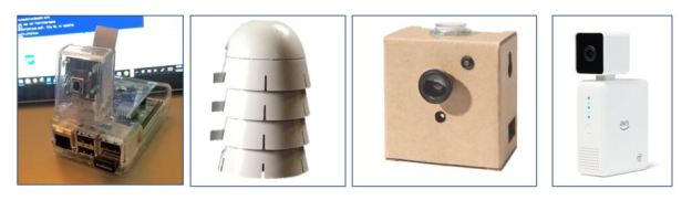
Figure 1.  From the left is a RaspberryPi with an attached camera, ANL Waggle array, the Google AIY vision kit and the AWS DeepLens.

The Pi system is, by far, the least capable with a quad core ARMv7 processor and 1 GB memory.   The Google vision kit has a Raspberry Pi Zero W (single core ARMv7 with 512MB memory) but the real power lies in the Google VisionBonnet which uses a version of the Movidius Myriad 2 vision processing chip which has 12 vector processing units and a dual core risc cpu.   The VisionBonnet runs TensorFlow from a collection of pretrained models.    DeepLens has a 4 megapixel camera, 8 GB memory, 16 GB storage and an intel Atom process and Gen9 graphics engine which supports model built with Amazon SageMaker that is pre-configured to run TensorFlow and Apache MXNet.

As we stated above many applications that run on the edge many must rely on the cloud if only for storing data to be analyzed off-line.   Others, such as many of our phone apps and smart speakers, use the cloud for backend computation and search.   It may be helpful to think of the computational capability of edge devices and the cloud as a single continuum of computational space and an application as an entity that has components distributed over both ends.   In fact, depending upon the circumstances parts of the computation may migrate from the cloud to the device or back to optimize performance.   As illustrated in Figure 2, AWS Greengrass accomplishes some of this by allow you to move Lambda “serverless” functions from the cloud to the device to form a network of long running functions that can interact with instruments and securely invoke AWS services.

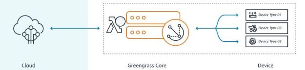
Figure 2.   AWS Greengrass allows us to push lambda functions from the cloud to the device and for these functions to communicate seamlessly with the cloud and other functions in other devices.  (Figure from https://aws.amazon.com/greengrass/ )

The Google vision kit is not available yet and DeepLens will ship later in the spring and we will review them when they arrive.   Here we will focus on a few simple experiments with the Raspberry Pi and return to these other devices in a later post.

Deep Learning Models and the Raspberry PI 3.

In a previous post we looked at several computer vision tasks that used the Pi in collaboration with cloud services.   These included simple object tracking and doing optical character recognition and search for information about book covers seen in an image.   In the following paragraphs we will focus on the more complex task of recognizing objects in images and we will try to understand the limitations and advantages of using the cloud as the backend computational resource.

As a benchmark for our experiments we use the Apache MXNet deep learning kit with a model based on the resnet 152-layer neural network that was trained on a  collection  of over a  10 million images and over 11 thousand labels.    We have packaged this MXNet with this model into a Docker container dbgannon/mxnet which we have used for these experiments.  (the details of the python code in the container are in the appendix to this blog.

Note: If you want to run this container and if you have dockerand Jupyter installed you can easily test the model with pictures of your own.  Just download the jupyter notebook send-to-mxnet-container.ipynb and follow the instructions there.

How fast can we do the image analysis (in image frames per second)?

Running the full resnet-152 model on an installed version  of MXNet  on more capable machines (Mac mini and the AWS Deeplearning AMI c5.4xlarge, no GPU)  yields an average performance of about 0.7 frame/sec.     Doing  the same experiment on the same machines, but using the docker container and a local version of the Jupyter notebook driver we see the performance degrade a bit to an average of about 0.69 frame/sec (on a benchmark set of images we described in the next paragraph).    With a GPU one should be able to go about 10 times faster.

For the timing tests we used a set of 20 images from the internet that we grabbed and reduced so they average about 25KB in size.  These are stored in the Edge device.  Loading one of these images takes about the same amount of time as grabbing a frame from the camera and reducing it to the same size.  Two of images from the benchmark set and the analysis output is shown in figure 3 below.

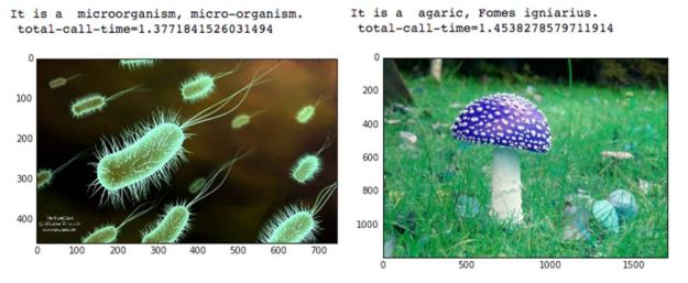
Figure 3. Two of the sample images together with the output analysis and call time.

How can we go faster on the Pi 3?   We are also able to install MXNet on the Pi 3, but it is a non-trivial task as you must build it from the source.   Deployment details are here, however, the resnet 152 model is too large for the 1MB memory of the Pi 3, so we need to find another approach.

The obvious answer is to use a much smaller model such as the Inception 21 layer network which has a model database of only 23MB (vs 310MB  for resnet 152), but it has only 1000 classes vs   the 11,000 of the full rennet 152. We installed Tensorflow on the Pi3. (there are excellent examples of using it for image analysis and recognition provided by Matthew Rubashkin of Silicon Valley Data Science.) We ran the Tensorflow Inception_2015_12_05 which fit in memory on the Pi.  Unfortunately, it was only able to reach 0.48 frames per second on the same image set described above.

To solve the, we need to go to the cloud.    In a manner similar to the Greengrass model,  we will have the Pi3 sample the camera and downsize the image and send it to the cloud for execution.   To test it we ran the MXNet container on a VM in AWS and pointed the Pi camera at various scenes.  The results are shown in Figure 4.

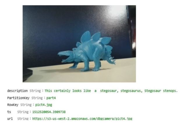
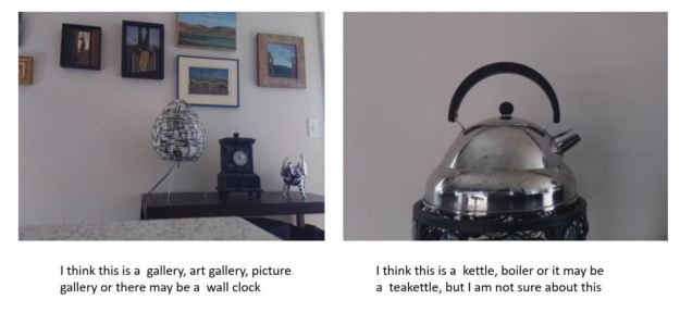
Figure 4.  The result for the toy dinosaur result is as it is logged into the AWS DynamoDB.   With the bottom two images show only the description string.

The output of the model gives us likelihood of various labels.  In a rather simple minded effort to be more conversational we translate the likelihood results as follows.  If a label X is  more than 75% likely  the container returns a value of “This certainly looks like a X”.   If the likely hood is less than less than 35%  it returns “I think this is an X, but I am not sure” (the code is below).    We look at the top 5 likely labels and they are listed in order.

The Pi device pushes jpeg images to AWS S3 as a blob.   It then pushes the metadata about the image (a blob name and time stamp) to the AWS Simple Queue Service.   We modified the MXNet container to wait for something to land in the queue. When this happens, it takes the image meta data and pulls the image from S3 and does the analysis and finally stores the result in an AWS DynamoDB table.

However we can only go as fast as we can push the images  and metadata to the cloud from the Pi device.   With repeated tries we can achieve 6 frames/sec.   To speed up the analysis to match this input stream we spun up a set of analyzers using the AWS Elastic Container Service (ECS).  The final configuration is shown in Figure 5.

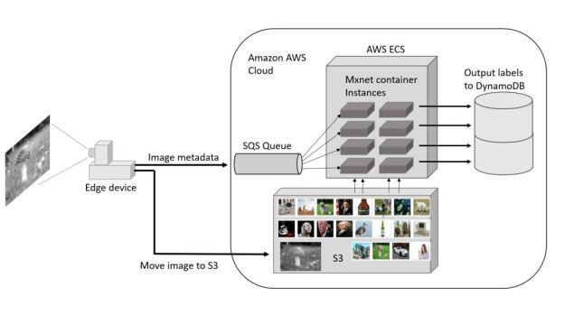
Figure 5.   The full Pi 3 to Cloud image recognition architecture. (The test dataset is shown in the tiny pictures in S3)

To conduct the experiments, we included a time stamp from the edge device with the image metadata. When the MXNet container puts the result in the DynamoDB table it includes another timestamp.  This allows us to compute the total time from image capture to result storage for each image in the stream. If the device sends the entire collection as fast as possible then the difference between the earliest recorded time stamp and the most recent gives us a good measure of how long it takes to complete the entire group.

While the Pi device was able to fill S3 and the queue at 6 frames a second having only one MXNet container instance yielded the result that the total throughput was only about 0.4 frames/sec.   The servers used to host the container are relatively small.   However, using the ECS it is trivial to boost the number of servers and instances.  Because of the size of the container instance is so large only one instance can fit on each of the 8 GB servers.   However as shown in Figure 6 we were able to match the device sending throughput with 16 servers/instances.  At this point messages in the queue were being consumed as fast as they were arriving. Using a more powerful device (a laptop with a core I7 processor) to send the images we were about to boost the input end up to just over 7  frames per second and that  was matched with 20 servers/instances.

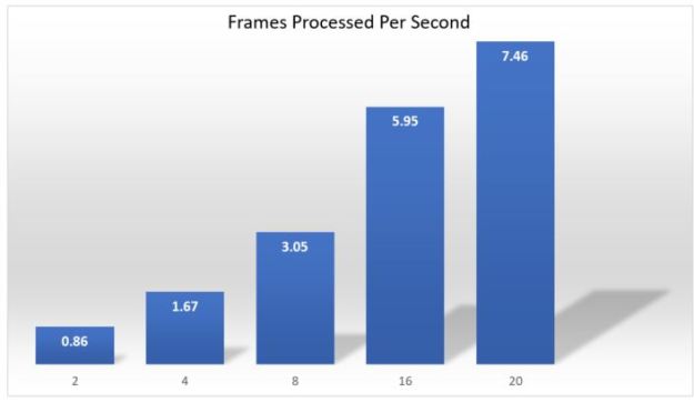
Figure 6.  Throughput in Frames/second measured from the Pi  device to the final results in the DynamoDB instance.   In the 20 instance case, a faster core I7 laptop was used to send the images.

Final Thoughts

This exercise does not fully explore the utility of AI method deployed at the edge or between the edge and the cloud.  Clearly this type of full object recognition at real-time frame rates is only possible if the edge device has sophisticated accelerator hardware.  On the other hand, there are many simple machine learning models that can be used for more limited applications.   Object motion tracking is one good example.  This can be done in real-time.    This is typically done by comparing a frame to a previous one and looking for the differences.   Suppose you need to invoke fire suppression when a fire is detected.   It would not be had to build a very simple network that can recognize fire but not simple movement of ordinary objects.   Such a network could be invoked whenever movement is detected and if it is fire the appropriate signal can be issued.

Face detection and recognition is possible with the right camera.   This was done  with the Microsoft Xbox-1 and it is now part of the Apple IPhone X.

There are, of course, limits to how much we want our devices to see and analyze what we are doing.   On the other hand it is clear that advances in automated scene analysis and “understanding” are moving very fast.   Driverless cars are here now and will be commonplace in a few years.   Relatively “smart” robots of various types are under development.   It is essential that we understand how the role of these machines in society can benefit the human condition along the lines of the open letter from many AI experts.

 

Notes about the MXNet container.

The code is based on a standard example of using MXNet to load a model and invoke it.   To initialize the model, the container first loads the model files into the root file system.  That part is not show here. The files are full-resnet-152-0000.parms (310MB), full-resnet-152-symbols.json (200KB) and full-synset.txt (300KB) . Once loaded into into memory  the full network is well over 2GB and the container requires over 4GB.

Following the load, the model is initialized.

import mxnet as mx
# 1) Load the pretrained model data
with open (' full-synset.txt ','r ') as f:
        synsets = [l.rstrip() for l in f]
sym, arg _params , aux_pa ram s = mx . model .load _checkpoint( 'full-resnet-152' ,0)
# 2) Build a model from the data
mod = mx.mod .Module (symbol =sym , context =mx. gpu ())
mod. bind ( for_training =False, data_shapes=[( 'data ',(1,3,224,224))])
mod. set_params ( arg_params , aux_params )

The function used for the prediction is very standard.  It takes three parameters: the image object, the model and synsnet (the picture labels).   The image is modified to fit the network and then fed to the forward end.  The output is a Numpy array which is sorted and the top five results are returned.

def predict(img, mod, synsets):
    img = cv2.resize(img, (224, 224))
    img = np.swapaxes(img, 0, 2)
    img = np.swapaxes(img, 1, 2)  
    img = img[np.newaxis, :] 
    mod.forward(Batch([mx.nd.array(img)]))
    prob = mod.get_outputs()[0].asnumpy()
    prob = np.squeeze(prob)
    a = np.argsort(prob)[::-1]
    result = []
    for i in a[0:5]:
          result.append( [ prob[i], synsets[i][synsets[i].find(' '):]])
    return result

The container runs as a webservice on port 8050 using the Python “Bottle” package.  When it receives a web POST message to “call_predict” it invokes the call_predict function below.  the image has been passed as a jpeg attachment with is extracted with the aid of the request package.   It is saved in a temporary file and then read by the OpenCV read function.  Unfortunately there was no way to avoid the save followed by read because of limitations to the API.  However we measured the cost of this step and it was less than 1% of the total time of the invocation.

The result of the predict function is a two dimensional array with each row consisting of a probability and the associated label.   The call returns the most likely labels as shown below.

@route('/call_predict', method='POST')
def call_predict():
    t0 = time.time()
    result = ''
    request.files.get('file').save('yyyy.jpg', 'wb')
    image = cv2.cvtColor(cv2.imread('yyyy.jpg'), cv2.COLOR_BGR2RGB)
    t1 = time.time()
    result = predict(image,  mod, synsets)
    t2 = time.time()
    answer = "i think this is a "+result[0][1]+" or it may be a "+result[1][1]
    if result[0][0] < 0.3:          answer  = answer+ ", but i am not sure about this."     if result[0][0] > 0.6:
         answer = "I see a "+result[0][1]+"."
    if result[0][0] > 0.75:
         answer = "This certainly looks like  a "+result[0][1]+"."
    answer = answer + " \n total-call-time="+str(t2-t0)
    return(answer)
run(host='0.0.0.0', port=8050)

The version of the MXNet container used in the ESC experiment replace the Bottle code and call_predict with loop that polls the message queue, pulls a blob from S3 and pushes the result to DynamoDB