
In Part 1 of this article we looked at how quantum computers are now beginning to appear as cloud hosted attached processors and we also looked at how one can go about programming them. The most important question that part 1 failed to address is why quantum computers are interesting? The most well-known uses of a quantum computer are for building interesting quantum chemistry models and for factoring large numbers to break cryptographic codes. The chemistry application was the original suggestion from Richard Feynman in 1981 for building a quantum computer. The factoring application is important, but it will only remain interesting until the cryptographers find better algorithms. Another application area that has received a lot of attention lately is applying quantum computing to machine learning (ML). This is not surprising. (Everything in AI is hot now, so quantum AI must be incandescent.)
Much of the published work on quantum ML is very theoretical and this article will try to provide pointers to some of the most interesting examples, but we will not go deep into the theory. However there are a few algorithms that run on the existing machines and we will illustrate one that has been provided by the IBM community. This algorithm builds a Support Vector Machines for binary classification and it runs on the IBM-Q system. More on that in the second half of this article.
The following is a list of papers and link that formed the source for the brief summary that follows. They are listed in chronological order. Several of these are excellent surveys with lots of technical details.
- Lloyd, M. Mohseni, and P. Rebentrost, Quantum algorithms for supervised and unsupervised machine learning, https://arxiv.org/abs/1307.0411 (2013)
- Lloyd, M. Mohseni, and P. Rebentrost, Quantum principal component analysis, https://arxiv.org/abs/1307.0401 (2013)
- Nathan Wiebey, Ashish Kapoor and Krysta M. Svore, Quantum Algorithms for Nearest-Neighbor Methods for Supervised and Unsupervised Learning, https://arxiv.org/abs/1401.2142 2014
- Maria Schuld, Ilya Sinayskiy and Francesco Petruccione, An introduction to quantum machine learning, https://arxiv.org/abs/1409.3097v1 2014
- Nathan Wiebe, Ashish Kapoor, and Krysta M. Svore, Quantum Deep Learning, https://arxiv.org/abs/1412.3489v2 2015
- Verdon, M. Broughton and J. Biamonte, A quantum algorithm to train neural networks using low-depth circuits, https://arxiv.org/pdf/1712.05304.pdf
- Jacob Biamonte, Peter Wittek, Nicola Pancotti, Patrick Rebentrost, Nathan Wiebe, Seth Lloyd, Quantum Machine Learning, https://arxiv.org/pdf/1611.09347v2.pdf 2018
- Seth Lloyd and Christian Weedbrook. Quantum generative adversarial learning, https://arxiv.org/pdf/1804.09139v1.pdf 2018
- Gao1, Z.-Y. Zhang, L.-M. Duan, A quantum machine learning algorithm based on generative models, http://advances.sciencemag.org/content/4/12/eaat9004.full, 2018
- Dawid Kopczyk “Quantum machine learning for data scientists” 2018
A Tour of Quantum ML Algorithms
The normal breakdown of machine learning algorithms is to divide it into 2 categories: supervised algorithms and unsupervised algorithms. Supervised algorithms include those where a quantity data and the “answers” are known, and we seek to build a model that will allow us to consider previously unseen data. These include simple regression, support vector machines (which we will consider in detail later), neural networks, restricted Boltzmann machines and deep learning classifiers. Unsupervised algorithms include clustering, dimensionality reduction and methods such as principle component analysis, and generative adversarial networks.
Because most of the work on quantum ML is theoretical the measure of success is based on complexity theory and the holy grail for quantum algorithms is a proof of exponential speed up of the quantum algorithm over the best sequential counterpart. In the case of the classical ML algorithms that run in polynomial time (as a function of input data size), an exponential speedup for a quantum algorithm would be one that runs in polylogarithmic time or less. But if the data input must be loaded into the quantum computer, then any sequential read of the data would require linear time and we cannot boast true exponential speed-up. One way around this is to assume the data has been preloaded into a “quantum random access memory” (qRAM). An alternative is to consider problems where the data is generated by an internal algorithm or a natural process.
A commentary in Nature by Scott Aaronson entitled “Read the fine print” (2015) points out that there are several difficulties with many quantum algorithms. These include the transformation of the data vector of dimension N into to log(N) qubits, the fact that the matrices must be well conditioned and the fact that the vector outputs may be difficult to read if they contain components that differ greatly in scale. In general, the “Quantum Supremacy” of a quantum algorithm may be theoretically true but it may be lost to fast classical algorithms in real applications if nasty constant factors dominate.
Looking at a Few Algorithms
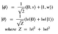
A frequent assumption about data is that it is composed of vectors of dimension N=2n. These may be real or complex values. Let v = {v1, v2, … , vN} be such a vector, then we assume we can imbed this into n qubits as
If this can be done, it has some nice properties that can be used in some important quantum subroutines in the quantum ML algorithms.
K-Means Algorithm
K-means is one of the standard classic ML unsupervised algorithms. It uses the vector-to-quantum vector map described above. If we define a second vector w in a similar way and then define
A bit of algebra will verify that
![]()
This implies we can compute Euclidian distance if we can compute |<ϴ | φ > |2 . It turns out there is a simple quantum circuit, called the swap-test that can help us estimate this value.
Given this distance algorithm and another standard subroutine called Grover’s algorithm (that allows us to pick the best from alternatives) we can build a K-means algorithm. The quantum advantage of this algorithm only show up when N is large because the complexity of the classical algorithm with M data points is O(MN) and with the quantum algorithm it is O(M log(N)).
Principal Component Analysis
PCA is based on finding the eigenvectors of the covariance matrix of a set of input vectors. The quantum version of this algorithm uses an important subroutine called quantum phase estimation, which is a method to find the eigenvalues of a unitary matrix. For unitary matrices the eigenvalues are always of the form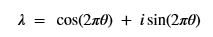
The algorithm computes the phase ϴ.
For PCA in general, we start with a set of vectors {vi , i = 1, M}. The jth component of vi can be thought of jth feature of the vector. To simplify the discussion let’s assume that mean of this feature is 0 for all M vectors. In otherwords, set vi = vi – 1/M*sum(vi, i=1,M). We are looking for eigenvalues and eigenvectors of the matrix C = Vt * V where V is the NxM matrix consisting the vectors {vi , I = 1, M}. Another way to describe C is by the fact that it is NxN with Ci, j = sum( vki* vk j , k =1,M). C is M times the covariance matrix for our set of normalized vectors. The eigenvectors of C form a new basis that diagonalizes C with the eigenvalues on the diagonal.
In the quantum algorithm we use the map of our vector data into the quantum space as above
Where we have also normalized each vector to unit length. Now we build the Hermitian operator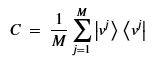
Expanding out the tensor product from the embedding representation we see this is precisely the quantum version of our covariance matrix. We can now turn this into a problem of finding the eigenvalues of a unitary matrix with the formula

The algorithm now can use phase estimation and other tricks to get to the eigenvectors and values. For the serious details see reference [7] and [10] above.
Neural Networks: RBMs and GANs
Paper [5] and [7] discuss approaches to quantum versions of restricted Boltzmann machines (RBMs). Unlike the standard feed-forward deep neural network used for classification tasks, RBMs are a type of generative neural network. This means that they can be used to build a model of the statistical distribution of observed data. Sampling from this distribution can give you new examples of “similar” data objects. For example, a picture of a human face that is like others but different, or a potential chemical compound for drug discovery research. The simplest form of a RBM is a two layer network with one layer which is the visible nodes (v1, v2, .. vm) and the other is called the hidden layer of nodes (h1, h2, …, hn). Each visible node is connected to each hidden node as shown in the figure below.
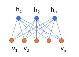
We assume that all the data are binary vectors of length m. We use each data sample to predict values for the hidden state using a sigmoid function and a set of weights wi,j connecting visible node i to hidden node j and an offset ai. What results is a conditional probably for h given v. Then given a sample of hidden states we project them back to the visible layer by a similar conditional probability function.

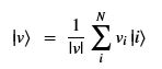
The joint probability for v and h is given by

Where the energy function is given by

Where Z is the normalizing sum. This distribution is the Boltzmann or Gibbs distribution. There are several quantum solutions. One is to us simulated annealing which can be done on a machine like the D-wave system. The other approach is to exploit a technique known as Gibbs sampling. One can use the quantum computers can draw unbiased samples from the Gibbs distribution, thereby allowing the probabilities P(v,h) to be computed by quantum sampling. It seems that this can be done with a relatively small number of qubits, but the reader should consult [5] to get the full picture.
Paper [9] considers the problem of creating quantum generative systems by starting with factor graphs and then then construct a quantum state that represents the distribution associated with the graph. They then show that this is conceptually more powerful that then factor graph approach.
RBMs are one of the original forms of neural networks. (One survey article calls them the “model T” of networks.) RBM are not used very often because other generative methods seem to work better. One such better method is the Generative Adversarial Network (GAN), in which two networks compete. We discussed GANS in a previous post. One network called the generator and its job is to generate sample data that will fool the other network, the discriminator. The discriminator’s job is to tell the real data samples from the fake. When the system converges the discriminator is correct half the time and it is wrong half of the time.
In paper [8] the authors generalize this to the quantum case by proposing three variations: both the discriminator are quantum systems, the discriminator is quantum and the generator is classical and the configuration where the discriminator is classical and the generator is quantum. They argue that for high dimensional data the quantum-quantum case may give exponential speed-up.
An Example: Support Vector Machines
To illustrate a simple quantum machine learning algorithm that runs on the IBM system we turn to a “classic” machine learning method known as Support Vector Machine (SVM). In general, an SVM can be used as a binary classifier of measurements of experiments where each experiment is represented by its features rendered as vector or point in Rn. For example, these might be measurements of cell images where we want to identify which cells are cancerous or it may be astronomical measurements of stars where we seek to determine which have planets. To understand the quantum version of SVM it is necessary to review the derivation of the classical case. In the simplest cases we can find a plane of dimension Rn-1 that separates the vectors (viewed as points) into two classes with the class on one side of the plane having the property we want and the class on the other side failing. These points with their label constitute the training set for the algorithm. In the case that n = 2, the plane is a line and the separator may look like figure 1a. The hyper plan can be described in terms of a normal vector w and an offset b. To determine if a point X in Rn is one side or the other of the plane, we evaluate
![]()
If f(X) > 0 then the point is on one side and if f(X) < 0 the point is on the other side.

Figure 1. a) on the left is a linear separator between the red and the blue points. b) on the right is an example without a linear separator.
The name “support vector” comes from the optimal properties of the separating hyperplane. The hyperplane is selected so that it maximized the distance from all the training examples. The distance of a point to the hyperplane is the minimum distance to the hyperplane. This minimum distance is on a vector from the plane to the point that is parallel to the normal vector of the plane. Those points whose distance is the minimum are called the support vectors. Because the plane maximizes the distance from all points, those minima must be equal. A bit of algebra will show the normal distance between the nearest points on one side of the plane and the nearest point on the other side is 2/||w||. (Hence to maximize the distance we want to minimize ||w||2/2.) Let {xi , yi} I = 1,N be the training points where yi = -1 if xi is in the negative class (making f(xi) < 0) and yi = 1 if xi is in the positive class ( f(xi) > 0) . To compute the values for w and b we first note that because f(X) is only + or -, we can scale both w and b by the same factor without changing the sign. Hence, we can assume
![]()
where equality happens only for the support vector points. To solve this problem of maximizing the minimum distance we are going to need to invoke a technique from math where we insert some new variables αi (known as Lagrange multipliers) and then compute
![]()
As stated above we need minimize ||w||/2 so we can minimize its square. Looking at the min term, we must compute

Taking the derivative with respect to w and b we get the minimum when

Substituting these into L we see we must compute

A look at L shows that when xi is not a support vector then the max cannot happen unless αi = 0. Numerically solving for the remaining αi’s we can compute b from the fact that for the K support vectors we have

The matrix

Is called the kernel matrix. The function f(X) now takes the form

The Nonlinear Case and the Kernel Trick
There are obviously many cases where a simple planar separator cannot be found. For example, Figure 1b contains two classes of points where the best separator is a circle. However, that does not mean there is no interesting combination of features that can be used to separate the classes with a plane if viewed in the right way. Let ϕ: Rn -> M be a mapping of out feature space into a space M of higher dimension. The goal is to find a function that spreads the data out so that we can apply the linear SVM case. All we require of M is that it be a Hilbert space where we can compute inner products in the usual way. If we define the function K(X,Y) = (ϕ(X) . ϕ(Y)) then our function f(X) above becomes

Where the ais and b are computed in the space M. To illustrate this idea let ϕ: R2-> R3 be given by the mapping ϕ(X) = (X[0], x[1], 3 – 0.35*||X||2) and look at the data from figure 1b, but now in 3D (figure 2). As can be seen the mapping moves the data points onto a paraboloid where the points inside the circle are in the positive half-space and the rest are below. It is now relatively easy to find a planar separator in R3.
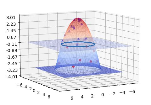
Figure 2. Kernel mapping R2 to R3 providing a planar separator for the data in Figure 1b.
When does this kernel function trick work? It turns out that it almost always does provided you can find the right mapping function. In fact the mapping function ϕ is not the important part. It is the function K(X,Y). As long as K is symmetric and positive semi-definite, then there is a function ϕ such that for every X and Y, K(X,Y) = (ϕ(X) . ϕ(Y)). But from the function f(X) above we see that we only need K and the inner product in M. As we shall see below M may be derived from quantum states.
Quantum Support Vector Machines.
We will look at the results of using a quantum SVM algorithm that run on the IBM quantum hardware. The complete mathematical details are in a paper by Vojtech Havlicek, et. al. entitled “Supervised learning with quantum enhanced feature spaces“ (https://arxiv.org/abs/1804.11326). They describe two algorithms. One of the algorithms is called a variational method and the other is a direct estimation of a quantum version of a Kernel function K(x,z). Because the later method is a tiny bit easier to explain we will follow that approach. There are two parts to this. We will work with examples with data in R2.
- First we construct a function φ from R2 into the space of positive semidefinite density matrices with unit trace. We need this function to be hard to compute classically so we can preserve the “quantum advantage”. We can then create a 2 qubit function from R2 as

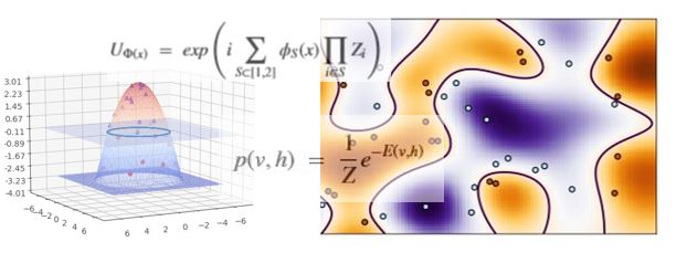
The transform Uφ(x) is the key to embedding out training and test data into 2 qubits. The exact definition involves selecting a set of nonlinear functions ϕS(x): R2 -> R where S ranges over the subsets of the set {1,2}. Given these functions, the unitary function Uφ(x) is defined as

Were Zi is the Pauli Z operator on the ith qubit.
To create our kernel function we look at
![]()
- This is almost the kernel, but not quite. What we define as the K(x,z) is related to the fidelities between x and z. To get that from the transition amplitudes above we measure this R times and if R is sufficiently large it will give us a good estimate.
Once we have computed Ki,j = K(xi, xj) for the training set we can now use the “classical” computer to calculate the support vector coefficients ai and offset b. To make predictions of f(Z) we now use the quantum computer to calculate K(xi , Z) for each of the support vectors and plug that into the formula above. The exact mathematical details for deriving φ are, of course, far more complicated and the reader should look at the full paper.
This example quantum support vector machine is available on-line for you to try out on IBM’s system. The code is simple because the details of the algorithm are buried in the qiskit.aqua libraries. To run the algorithm, we create a very small sample dataset from their library “add_hoc_data” and extract training and testing files.

There are two ways to run the algorithms. One way is a 3-line invocation of the prepackaged algorithm Below is the “programmers” which shows a few more details. This shows that we are using the qasm_simulator with 2 qubits where qubit 0 is connected to qubit 1 on the simulated hardware (this reflects the actual hardware). We create an instance and train it with 1024 “shots” (R above).

We can next print the kernel matrix and the results of the test.

Using the programming method, we can directly invoke the predict method on our trained model. We can use this to show a map of the regions of the quantum support “projected” to the 2-D plane of the sample data. We do this by running the predict function on 10000 points in the plane. And plot this as a map and then add the training points.

The resulting image is below. As you can see, the dark blue areas capture the orange data points and the lighter orange areas capture the light blue data points.

It is interesting to compare this result to running this with the Scikit SVM library. Using the library is very simple. Converting the data set from the quantum algorithm to one we can give to the Scikit library as vectors X and Y, we have

The Kernel function in this case is one of the standard kernels: RBF. Plotting the projection of the support surface wit the 2-D plain we see the image below.

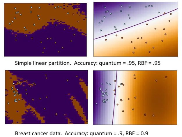
The match to the training data is perfect, but in this case the accuracy is only 0.6. We tried two additional test. The first was a simple linear partition along the line y = 0.6*x-0.2 with 20 points above the line and 20 below. In this case the quantum computation did not as well at first, but after several attempts with different data sets, it achieved a score of .95 and the Scipy RBF kernel also got a score of 0.95. The figure below illustrates the regions captured by both algorithms. We also used another example from their data collection consisting of breast cancer cases. The data was relatively high dimensional, so they projected it onto the 2 principal axes. In this case the quantum and the Scipy RBF both achieved an accuracy of 0.9.
After numerous experiments we found that the quantum algorithm was unstable in that there were several cases that caused it to fail spectacularly (accuracy = 0.4). However, when it worked it worked very well. The experiments above were with very tiny data sets that were selected so the results could be easily visualized. A real test would require data sets 100 to 1000 time larger.
Conclusions
Quantum computers are now appearing as cloud-based resources and when used with algorithms that exploit the quantum subsystem and classical computer working together, real breakthroughs may be possible. In the area of AI and machine learning, the current work is primarily very theoretical, and we hope that we have given the interested reader pointers to some of the recent papers. We took a deep dive into one classical algorithm, support vector machines, and illustrated it with a code that runs on the IBM-Q system. Our results were impressive in terms of accuracy, but we did not see speed-up over the classical algorithm because of the small size and dimensionality of the data sets.
The current crop of algorithms will need improvements if they are to show substantial speed-up on real world problems. In particular, the mapping from real data to quantum states will need to improve. But this will be an area where we can expect to see substantial investment and research energy over the next few years.
