
Abstract. Probabilistic programming languages (PPLs) allow us to model the observed behavior of probabilistic systems in terms its underlying latent variables. Using these models, the PPL provides tools to make inferences concerning the latent variables that give rise to specific observed behaviors. In this short report, we look at two such programming languages: Gen, a language based on Julia from a team at MIT and PyProb which is based on Python and Torch from the Probabilistic Programming Group at the University of Oxford. These are not the only PPls nor are they the first, but they illustrate the concepts nicely and they are easy to describe. To fully understand the concepts behind these systems requires a deep mathematical exploration of Bayesian statistics and we won’t go there in this report. We will use a bit of math, but the beauty of these languages is that you can get results with a light overview of the concepts.
Introduction
In science we build theories that tell us how nature works. We then construct experiments that allow us to test our theories. Often the information we want to learn from the experiments is not directly observable from the results and we must infer it from what we measure. For example, consider the problem of inferring the masses of subatomic particles based on the results of collider experiments, or inferring the distribution of dark matter from the gravitational lensing effects on nearby galaxies, or finding share values that optimize financial portfolios subject to market risks, or unravelling complex models of gene expression that manifest as disease.
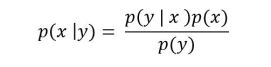
Often our theoretical models lead us to build simulation systems which generate values we can compare to the experimental observations. The simulation systems are often programs that draw possible values for unknowns, call them x, from random number generators and these simulations use these values to generate outcomes y. In other words, given values for x, our simulation is a “generative” function F which produces values y = F(x). If our experiments give us values y’, we can think of the inference task as solving the inverse problem x = F-1(y’), i.e. finding values for the hidden variables x that give rise to the observed outcomes y’. The more mathematical way to say this to say that our simulation gives us a probability distribution of values of y given the distribution associated with the random draws for x, which we write as p(y | x ). What we are interested in is the “posterior” probability p(x | y’) which is the distribution of x given the evidence y’. In other words, we want samples for values of x that generate values close to our experimental values y’. These probabilities are related by Bayes Theorem as
Without going into more of the probability theory associated with this equation, suffice it to say that the right-hand side of this equation can be very difficult to compute when F is associated with a simulation code. To get a feel for how we can approach this problem, consider the function F defined by our program as a generative process: each time we run the program it makes a series of decisions based on random x values it draws and then generates a value for y. What we will do is methodically trace the program, logging the values of x and the resulting ys. To get a good feel for the behavior of the program, we will do this a million time.
Begin by labeling each point in the program where a random value is drawn. Suppose we now trace the flow of the program so that each time a new random value is drawn we record the program point and the value drawn. As shown in Figure 1, we define a trace of the program to be the sequence [(a1, x1), (a2, x2), …(an, xn), y] of program address points and random values we encounter along the way.
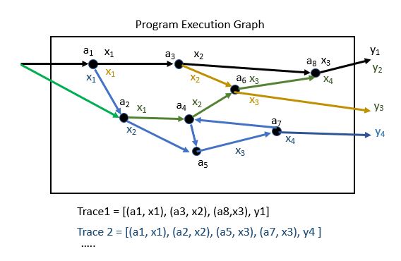
Figure 1. Illustration of tracing random number draws from a simulation program. A trace is composed of a list of address, value tuples in the order they are encountered. ( If there are loops in the program we add an instance count to the tuple.)
If we can trace all the paths through the program and compute the probabilities of their traversal, we could begin to approximate the joint distribution p(x,y)=p(y|x)*p(y) but given that the x’s are drawn from continuous distributions this may be computationally infeasible. If we want to find those traces that lead to values of y near to y’, we need to use search algorithms that allow us to modify the x’s to construct the right traces. We will say a bit more about these algorithms later, but this is enough to introduce some of the programming language ideas.
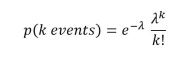
To illustrate our two probabilistic programming languages, we will use an example from the book “Bayesian Methods for Hackers” by Cameron Davidson-Pilon. (There are some excellent on-line resources for the book. This includes Jupyter notebooks for each chapter that have been done with two other PPLs: PyMC3 and Tensorflow Probability.) The example comes from chapter 1. It concerns the logs of text messages from a user. More specifically, it is the number of text messages sent per day over a period of 74 days. Figure 2 shows bar graph of the daily message traffic. Looking at the data, Davidson-Pilon made a conjecture that the traffic changes in some way at some point so that the second half of the time period has a qualitative difference from the first half. Data like this is usually Poisson distributed. If so, there is an average event rate such that the probability of k events in a single time slot is given by
If there really are two separate distributions the let us say the event rate is for the first half and for the second half and a day such that for all days before that date the first rate applies and it is the second rate after that. (This is all very well explained in the Davidson-Pilon book and you should look at the solution there that uses PPL PyMC3. The solutions here are modeled on that one.)
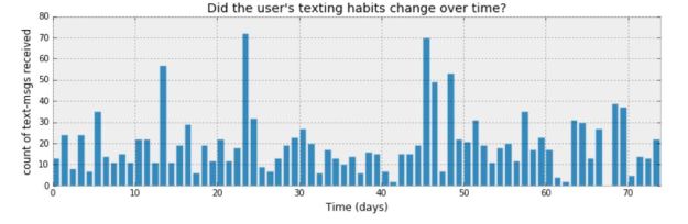
Figure 2. From Chapter 1 of “Bayesian Methods for Hackers” by Cameron Davidson-Pilon.
Gen
Gen is a language that is built on top of Julia and Tensorflow by Marco Cusumano-Towner, Feras A Saad, Alexander K Lew and Vikash K Mansinghka at MIT and described in their recent POPL paper [1]. In addition they have a complete on-line resource where you can download the package and read tutorials.
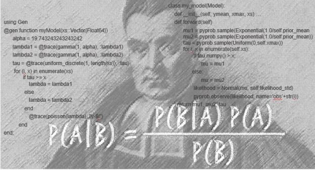
We gave a brief introduction to Julia in a previous article, but it should not be hard to understand the following even if you have never used Julia. To cast this computation into Gen we need to build a model that captures the discussion above. Shown below we call it myModel.
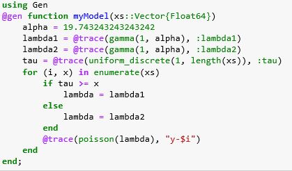
The first thing you notice about this code are the special annotations @gen and @trace. This tells the Gen system that this is a generative model and that it will be compiled so that we can gather the execution traces that we discussed above. We explicitly identify the random variables we want traced by the @trace annotation. The argument to the function is a vector xs of time intervals from 1 to 74. We create it when we read the data from Figure 2 from a csv file (which is shown in detail in the full Jupyter notebook for this example). Specifically, xs = [1.0, 2.0, 3.0 …, 74.0] and we set a vector ys so that ys[i] is the number of text messages on day i.
If our model process is driven by a Poisson to generate y value, then the math says we should assume that the time interval between events is exponentially distributed. Gen does not have an exponential distribution function, but it does have a Gamma distribution and gamma(1, alpha) = exponential(1.0/alpha) . The statement
lambda1 = @trace(gamma(1, alpha), :lambda1)
tells Gen to pull lambda1 values from the exponential with mean alpha and we have initialized alpha to be the mean of the ys values (which we had previously computed to be 19.74…). Finally note we have used a special Julia labeling technique :variable-name to label this to be :lambda1. This is effectively the address in the code of the random number draw that we will use to build traces.
We draw tau from a uniform distribution (and trace and label it) and then for each x[i] <= tau we assign the variable lambda to lambda1 and for each x[i] > tau we assign lambda to lambda2. We use that value of lambda to draw a variable from the Poisson distribution and label that draw with a string “y-i”.
We can now generate full traces of our model using the Gen function simulate() and pull values from the traces with the get_choices() function as shown below.
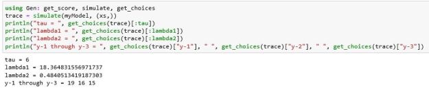
The values for the random variable draws are from our unconstrained model, i.e. they reflect the joint probability p(x,y) and not the desired posterior probability p(x | y’) that we seek. To reach that goal we need to run our model so that we can constrain the y values to y’ and search for those traces that lead the model in that direction. For that we will use a variation of a Markov Chain Monte Carlo (MCMC) method called Metropolis-Hastings (MH). There is a great deal of on-line literature about MH so we won’t go into it here, but the basic idea is simple. We start with a trace and then make some random mods to the variable draws. If those mods improve the result, we continue. If not, we reject it and try again. This is a great oversimplification, but Gen and the other PPLs provide library functions that allow us to easily use MH (and other methods.) The code below shows the how we can invoke this to make inferences.
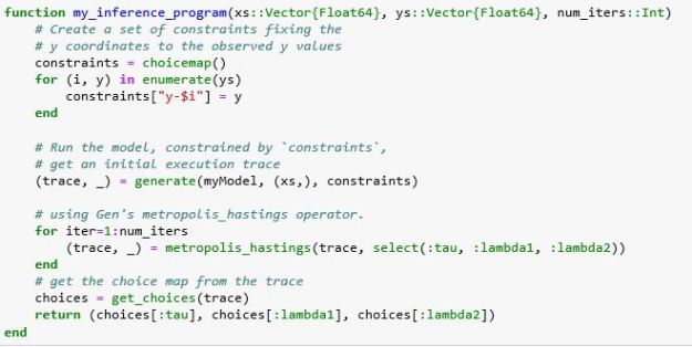
The inference program creates a map from the labels for the y values to the actual constraints from our data. It then generates an initial trace and iteratively applies the MH algorithm to improve the trace. It then returns the choices for our three variables from the final trace. Running the algorithm for a large number of iterations yields the result below.
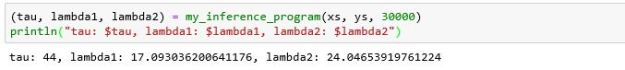
This result is just one sample from the posterior probabilities. If we repeat this 100 times we can get a good look at the distribution of values. Histograms of these values are shown below in Figure 3.
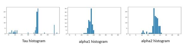
Figure 3. Histograms of the tau and lambda values. While difficult to read, the values are clustered near 44, 18, 24 respectively.
If we compare these results to the Davidson-Pilon book results which used the PyMC3 (and Tensorflow Probability) PPL, we see they are almost identical with the exception of the values of tau near 70 and 5. We expect these extreme values represent traces where the original hypothesis of two separate alphas was not well supported.
There is a great deal about Gen we have not covered here including combinators which allow us to compose generative function models together. In addition, we have not used one of the important inference mechanisms called importance sampling. We shall return to that topic later.
PyProb
Tuan Anh Le, Atılım Günes Baydin, Frank Wood first published an article about PyProb in 2017 [3] and another very important paper was released in 2019 entitled “Etalumis: Bringing Probabilistic Programming to Scientific Simulators at Scale” [4] which we will describe in greater detail later. PyProb is built on top of the deep learning toolkit PyTorch which was developed and released by Facebook research.
Many concepts of PyProb are very similar to Gen, but PyProb is Python based so it looks a bit different. Our generative model in this case is an instance of a Python class as shown below. The main requirement of the is that it subclass Model and have a method called forward() that describes how to generate our traces. Instead of the trace annotation used in Gen, we use PyProb sample and observe functions. The random number variables in PyProb are all Torch tensors, so to we need to apply the method numpy() to extract values. The functions Normal, Exponential and Uniform are all imported from PyProb. Other than that, our generator looks identical to the Gen example.
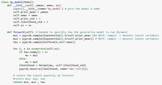
Also note we have used the name mu1 and mu2 instead of alpha1 and alpha2 (for no good reason.) Running the MH algorithm on this model is almost identical to doing it in Gen.
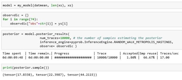
Again, this is just a sample from the posterior. You will notice that the posterior result function also tells us what percent of the traces were accepted by the MH algorithm. PyProb has its own histogram methods and the results are shown in Figure 4 below. The legend in the figure is difficult to read. It shows that the tau value is clusters near 44 with a few traces showing between 5 and 10. The mu1 values are near 17 and mu2 values are near 23. In other words, this agrees with our Gen results and the PyMC3 results in the Davidson-Pilon book.
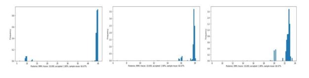
Figure 4. Histogram of tau, mu1 and mu2 values.
Building a PyProb Inference LSTM network.
There are several additional features of PyProb that are worth describing. While several of these are also part of Gen, they seem to be better developed in PyProb. More specifically PyProb has been designed so that our generative model can be derived from an existing scientific simulation code and it has an additional inference method, called Inference Compilation, in which a deep recurrent neural network is constructed and trained so that it can give us a very good approximation of our posterior distribution. In fact the neural network is a Long Short Term Memory (LSTM) network that that is trained using traces from out model or simulation code. The training, which can take a long time, produces a “distribution” q(x | y) that approximates our desired p(x | y). More of the details are given in the paper “Inference Compilation and Universal Probabilistic Programming” by Anh le, Gunes Baydin and Wood [3]. Once trained, as sketched in Figure 5, when the network is fed our target constraints y’ and trace addresses, the network will generate the sequence of components needed to make q(x|y= y’).
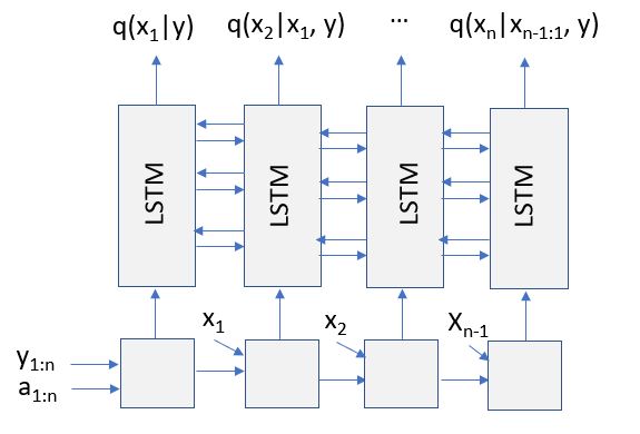
Figure 5. Recurrent NNet compiled and trained from model. (see [3, 4])
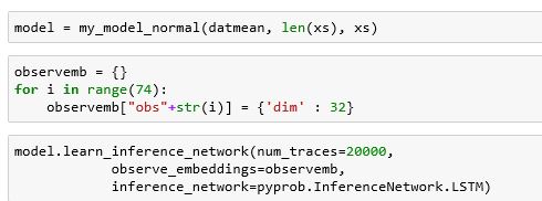
Building and training the network is almost automatic. We had one problem. The compiler does not support the exponential distribution yet, so we replaced it with a normal distribution. To do create and train the RNN was one function call as shown below.
Once trained (which took a long time), using it was also easy. In this case we use the importance sampling algorithm which is described in reference [3] and elsewhere.
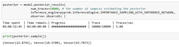
Figure 6 illustrates the histograms of values drawn from the posterior.
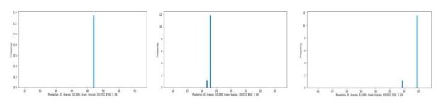
Figure 6. Using the trained network with our data. As can be seen, the variance of the results is very small compared to the MH algorithm.
The fact that the training and evaluation took so much longer with our trivial example is not important, because the scalability of importance sampling using the compiled LSTM network. In the excellent paper “Etalumis: Bringing Probabilistic Programming to Scientific Simulators at Scale” [4] Güneş Baydin, et. Al. describe the use of PyProb with a very large simulation code that models LHC experiments involving the decay of the tau lepton. They used 1024 nodes of the Cori supercomputer at LBNL to train and run their IC system. To do this required using PyProb’s ability to link a PyProb model to a C++ program. Using the IC LSTM network, they were able achieve a speed-up of over 200 over a baseline MCMC algorithm. The paper describes the details of the implementation and testing.
Conclusion
The goal of this paper was to introduce the basic ideas behind Probabilistic Programming Languages by way of two relatively new PPLs, Gen and PyProb. The example we used was trivial, but it illustrated the concepts and showed how the basic ideas were expressed (in very similar terms) in both languages. Both languages are relatively new and they implementations are not yet fully mature. However, we are certain that probabilistic programming will become a standard tool of data science in the future. We have put the source Jupyter Notebooks for both examples on GitHub. Follow the installation notes for Gen and PyProb on their respective webpages and these should work fine.
https://github.com/dbgannon/probablistic-programming
The traditional way computer science is taught involves the study of algorithms, based on cold, hard logic which, when turned into software, runs in a deterministic path from input to output. The idea of running a program backward from output to the input does not make sense. You can’t “unsort” a list of number. The problem is even more complicated if our program is a scientific simulation or data science involving machine learning. In these cases, we learn to think about the results of a computation as representatives of internally generated probability distributions.
Some of the most interesting recent applications of AI to science have been the result of work on generative neural networks. These systems are trained to perfectly mimic the statistical distribution of scientific data sets. They can allow us to build “fake” human faces or perfect, but artificial spiral galaxies, or mimic the results of laboratory experiments. They can be extremely useful but, in the case of science, they tell us little about the underlying laws of nature. PPLs allow us to begin to rescue the underlying science in the generative computation.
References
Some of these are link. Two can be found on arXiv and the Gen paper can be found in the ACM archive.
- Gen: A General-Purpose Probabilistic Programming System with Programmable Inference. Cusumano-Towner, M. F.; Saad, F. A.; Lew, A.; and Mansinghka, V. K. In Proceedings of the 40th ACM SIGPLAN Conference on Programming Language Design and Implementation (PLDI ‘19).
- https://github.com/probprog/pyprob
- Tuan Anh Le, Atılım Günes Baydin, Frank Wood, Inference Compilation and Universal Probabilistic Programming, arXiv:1610.09900v2
- Güneş Baydin, et al, “Etalumis: Bringing Probabilistic Programming to Scientific Simulators at Scale”, arXiv:1907.03382v1
- https://camdavidsonpilon.github.io/Probabilistic-Programming-and-Bayesian-Methods-for-Hackers/
- ABC–Fun: A Probabilistic Programming Language for Biology https://link.springer.com/chapter/10.1007/978-3-642-40708-6_12
- https://knect365.com/quantminds/article/7e2e4aaa-4115-42ca-8b84-4f4512e07974/deep-probabilistic-programming-for-financial-modeling
