Abstract
This short report describes the core features of the Ray Distributed Object framework. To illustrate Ray’s actor model, we construct a simple microservice-like application with a web server frontend. We compare Ray to similar features in Parsl and provide a small performance analysis. We also provide an illustration of how Ray Tune can optimize the hyperparameter of a neural network.
Introduction
Ray is a distributed object framework first developed by the amazingly productive Berkeley RISE Lab. It consists of a number of significant components beyond the core distributed object system including a cluster builder and autoscaler, a webserver framework, a library for hyperparameter tuning, a scalable reinforcement learning library and a set of wrappers for distributed ML training and much more. Ray has been deeply integrated with many standard tools such as Torch, Tensorflow, Scikit-learn, XGBoost, Dask, Spark and Pandas. In this short note we will only look at the basic cluster, distributed object system and webserver and the Ray Tune hyperparameter optimizer. We also contrast the basics of Ray with Parsl which we described in a previous post. Both Ray and Parsl are designed to be used in clusters of nodes or a multi-core server. They overlap in many ways. Both have Python bindings and make heavy use of futures for the parallel execution of functions and they both work well with Kubernetes, but as we shall see the also differ in several important respects. Ray supports an extensive and flexible actor model, while Parsl is primarily functional. Parsl is arguably more portable as it supports massive supercomputers in addition to cloud cluster models.
In the next section we will look at Ray basics and an actor example. We will follow that with the comparison the Parsl and discuss several additional Ray features. Finally, we turn to Ray Tune, the hyperparameter tuning system built on top of Ray.
Ray Basics
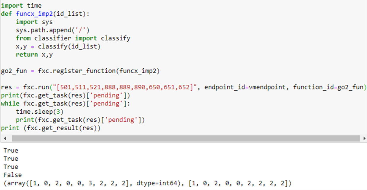
Ray is designed to exploit the parallelism in large scale distributed applications and, like Parsl and Dask, it uses the concept of futures as a fundamental mechanism. Futures are object returned from function invocations that are placeholders for “future” returned values. The calling context can go about other business while the function is executing in another thread, perhaps on another machine. When the calling function needs the actual value computed by the function it makes a special call and suspends until the value is ready. Ray is easy to install on your laptop. Here is a trivial example.

The result is

As you can see, the “remote” invocation of f returns immediately with the object reference for the future value, but the actual returned value is not available until 2 seconds later. The calling thread is free to do other work before it invokes ray.get(future) to wait for the value.
As stated above, Parsl uses the same mechanism. Here is the same program fragment in Parsl.

Ray Clusters and Actors
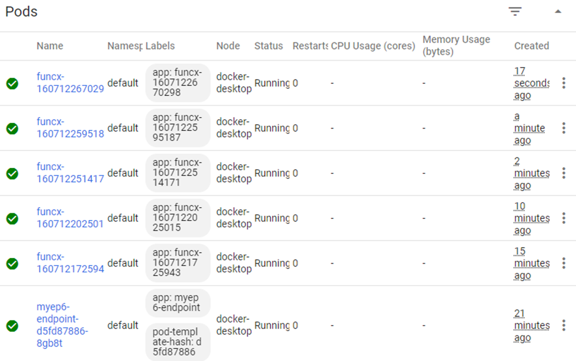
Ray is designed to manage run in ray clusters which can be launched on a single multicore node, a cluster of servers or as pods in Kubernetes. In the trivial example above we started a small Ray environment with ray.init() but that goes away when the program exits. To create an actual cluster on a single machine we can issue the command
$ ray start -–head
If our program now uses ray.init(address=’auto’) for the initialization the program is running in the new ray cluster. Now, when the program exits, some of the objects it created can persist in the cluster. More specifically consider the case of Actors which, in Ray, are instances of classes that have persistent internal state and methods that may be invoked remotely.
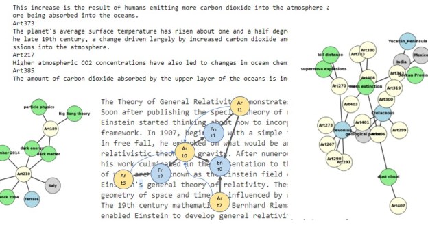
To illustrate Ray actors and the Ray web server will now describe an “application” that dynamically builds a small hierarchy of actors. This application will classify documents based on the document title. It will first classify them into top-level topics and, for each top-level topic subdivided further into subtopic as shown in Figure 1. Our goal here is not actually to classify documents, but to illustrate how Ray works and how we might find ways to exploit parallelism. Our top-level topics are “math”, “physics”, “compsci”, “bio” and “finance”. Each of these will have subtopics. For example “math” has subtopics, “analysis”, “algebra” and “topology”.

Figure 1. Tree of topics and a partial list of subtopics
We will create an actor for each top-level topic that will hold lists of article titles associated with the subtopics. We will call these actors SubClassifiers and they are each instances of the following class.

We can create an instance of the “math” actor with the call
cl = SubClassifier.options(name=”math”, lifetime=”detached”).remote(“math”)
There are several things that are happening here. The SubClassifier initializer is “remotely” called with the topic “math”. The initializer reads a configuration file (read_config) to load the subtopic names for the topic “math”. From that the subtopic dictionaries are constructed. We have also included an option that instructs that this instance to be “detached” and live in the cluster beyond the lifetime of the program that created it. And it shall have the name “math”. Another program running in the cluster can access this actor with the call
math_actor = ray.get_actor(“math”)
Another program running in the same Ray cluster can now add new titles to the “math” sub-classifier with the call
math_actor.send.remote(title)
In an ideal version of this program we will use a clever machine learning method to extract the subtopics, but here we will simply use a tag attached to the title. This is accomplished by the function split_titles()
We can return the contents of the sub-classifier dictionaries with
print(math_actor.get_classification.remote())
A Full “Classifier” Actor Network.
To illustrate how we can deploy a set of actors to make the set of microservice-like actors we will create a “document classifier” actor that allocates document titles to the SubClassifier actors. We first classify the document into the top-level categories “math”, “physics”, “compsci”, “bio” and “finance”, and then send them to the corresponding SubClassifier actor.
The Classifier actor is shown below. It works as follows. A classifier instance has a method “send(title)” which uses the utility function split_titles to extract the top-level category of the document. But to get the subcategory we need to discover and attach the subcategory topic tag to the title. A separate function compute_subclass does that. For each top-level category, we get the actor instance by name, or if it does not exist yet, we create it. Because computing the subclass may require the computational effort of a ML algorithm, we invoke compute_subclass as remote and store the future to that computation in a list and go on and process the next title. If the list reaches a reasonable limit (given by the parameter queue_size) we empty the list and start again. Emptying the list requires waiting until all futures are resolved. This is also a way to throttle concurrency.
By varying the list capacity, we can explore the potential for concurrency. If queue_size == 0, the documents will be handled sequentially. If queue_size == 10 there can be as many of 10 documents being processed concurrently. We shall see by experiments below what levels of concurrency we can obtain.

In the ideal version of this program the function compute_subclass invoked a ML model to compute the subclassification of the document, but for our experiments here, we will cheat because we are interested in measuring potential concurrency. In fact the subclassification of the document is done by the split_titles() function in the SubClassifier actor. ( The document titles we are using all come from ArXiv and have a top level tag and subclass already attached. For example, the title ‘Spectral Measures on Locally Fields [math.FA]’ which is math with subtopic analysis. )
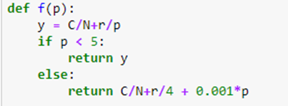
The simplified function is shown below. The work is simulated by a sleep command. We will use different sleep values for the final analysis.

The Ray Serve webserver
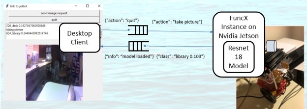
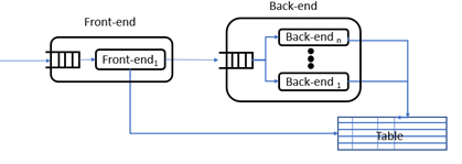
To complete the picture we need a way to feed documents to top-level classifier. We do that by putting a webserver in front and using another program outside the cluster to send documents to the server as as fast as possible. The diagram in Figure 2 below illustrates our “application”.

Figure 2. The microservice-like collection of Ray actors and function invocations. The clients send titles to the webserver “server” as http put requests. The server makes remote calls to the classifier instance which spawns compute_subclass invocations (labeled “classify()” here) and these invoke the send method on the subclassifiers.
The ray serve library is defined by backend objects and web endpoints. In our case the backend object is an instance of the class server.

Note that this is not a ray.remote class. Once Ray Serve creates an instance of the server which, in turn grabs an instance of the Classifier actor). The Server object has an async/await coroutine that is now used in the Python version of ASGI, the Asynchronous Server Gateway Interface. The call function invokes the send operation on the classifier. To create and tie the backend to the endpoint we do the following.

We can invoke this with

Serve is very flexible. You can have more than one backend object tied to the same endpoint and you can specify what fraction of the incoming traffic goes to each backend.
Some performance results
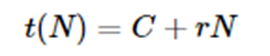
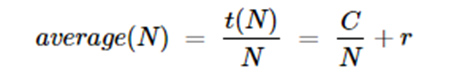
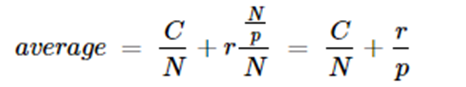
One can ask the question what is the performance implication of the parallel compute_subclass operations? The amount of parallelism is defined by the parameter queue_size. It is also limited by the size of the ray cluster and the amount of work compute_subclass does before terminating. In our simple example the “work” is the length of time the function sleeps. We ran the following experiments on AWS with a single multicore server with 16 virtual cores. Setting queue_size to 0 make the operation serial and we could measure the time per web invocation for the sleep time. For a sleep of t=3 seconds the round trip time per innovation was an average of 3.4 seconds. For t=5, the time was 5.4 and for t=7 it was 7.4. The overhead of just posting the data and returning was 0.12 seconds. Hence beyond sleeping there is about .28 seconds of ray processing overhead per document. We can now try different queue sizes and compute speed-up over the sequential time.

Figure 3. Speed up over sequential for 40 documents sent to the server.
These are not the most scientific results: each measurement was repeated only 3 times. However, the full code available for tests of your own. The maximum speed-up was 9.4 when the worker delay was 7 seconds and the queue length was 20. The code and data are in Github.
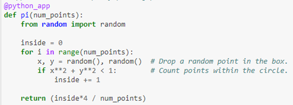
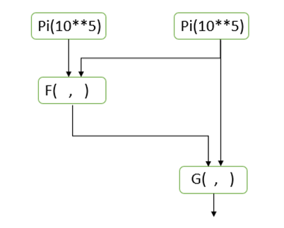
Another simple test that involves real computation is to compute the value of Pi in parallel. This involves no I/O so the core is truly busy computing. The algorithm is the classic Monte Carlo method of throwing X dots into a square 2 on a size and counting the number that land inside the unit circle. The fraction inside the circle is Pi/4. In our case we set X to 106 and compute the average of 100 such trials. The function to compute Pi is

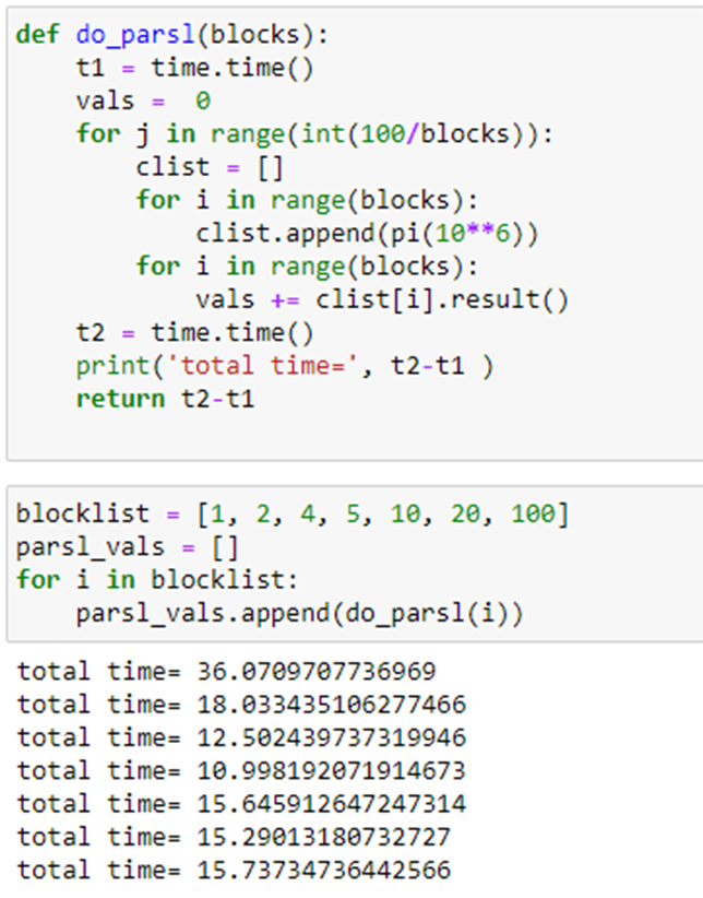
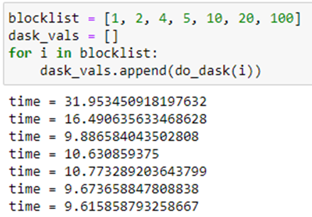
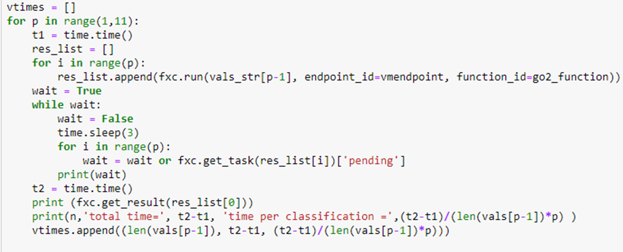
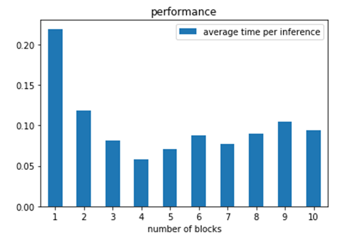
The program that does the test is shown below. It partitions the 100 Pi(10**6) tasks in blocks and each block will be executed by a single thread.

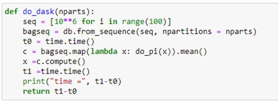
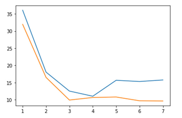
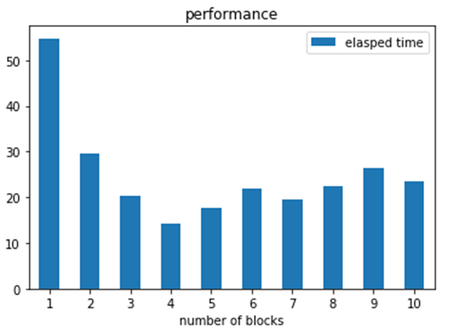
As can be seen the best time is when we compute 100 independent blocks. The sequential time is when it is computed as a sequential series of 100 Pi tasks. The speedup is 9.56. We also did the same computation using Dask and Parsl. In the chart below we show the relative performance .We also did the same computation using Dask and Parsl. The graph shows the execution time on the vertical axis and the horizontal is the block sizes 4, 5, 10, 20, 100. As you can see Dask is fastest but Ray in about the same when we have 100 blocks in parallel.

Figure 4. Execution time of 100 invocations of Pi(10**6). Blue=Parsl, Green=Ray and Orange=Dask.
More Ray
Modin
One interesting extension of Ray is Modin, a drop-in replacement for Pandas. Data scientists using Python have, to a large extent, settled on Pandas as a de facto standard for data manipulation. Unfortunately, Pandas does not scale well. Other alternatives out there are Dask DataFrames, Vaex, and the NVIDIA-backed RAPIDS tools. For a comparison see Scaling Pandas: Dask vs Ray vs Modin vs Vaex vs RAPIDS (datarevenue.com) and the Modin view of Scaling Pandas.
There are two important features of Modin. First is the fact that it is a drop-in replacement for Pandas. Modin duplicates 80% of the massive Pandas API including all of the most commonly used functions and it defaults to the original Pandas versions for the rest. This means you only need to change one line:
import pandas as pd
to
import modin.pandas as pd
and your program will run as before. The second important feature of Modin is performance. Modin’s approach is based on an underlying algebra of operators that can be combined to build the pandas library. They also make heavy use of lessons learned in the design of very large databases. In our own experiments with Modin on the same multicore server used in the experiments above Modin performed between 2 time and 8 times better for standard Pandas tasks. However, it underperformed Pandas for a few. Where Modin performance really shines is on DataFrames that are many 10s of gigabytes in size running on Ray clusters of hundreds of cores. We did not verify this claim, but the details are in the original Modin paper cited above.
Ray Tune: Scalable Hyperparameter Tuning
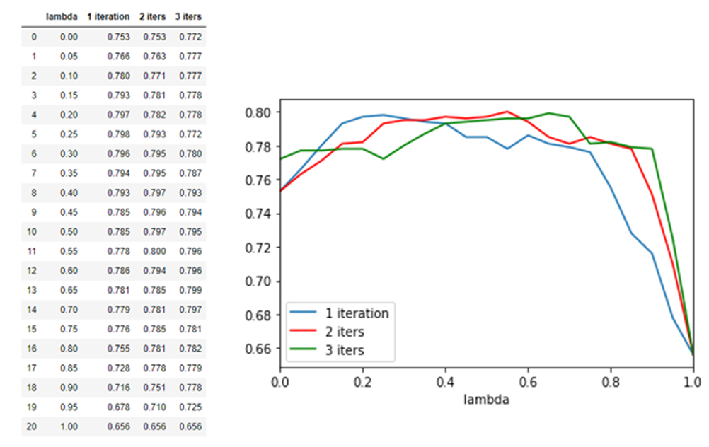
Ray Tune is one of the most used Ray subsystems. Tune is a framework for using parallelism to tune the hyperparameters of a ML model. The importance of hyperparameter optimization is often overlooked when explaining ML algorithm. The goal is to turn a good ML model into a great ML model. Ray Tune is a system to use asynchronous parallelism to explore a parameter configuration space to find the set of parameters that yield the most accurate model given the test and training data. We will Illustrate Tune with a simple example. The following neural network has two parameters: l1 and l2.

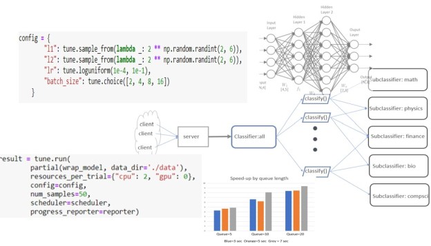
These parameters describe the shape of the linear transforms at each of the three layers of the network. When training the network, we can easily isolate two more parameters: the learning rate and the batch size. We can describe this parameter space in tune with the following.

This says that l1 and l2 are powers of 2 between 4 and 64 and the learning rate lr is drawn from the log uniform distribution and the batch size is one of those listed. Tune will extract instances of the configuration parameters and train the model with each instance by using Ray’s asynchronous concurrent execution.
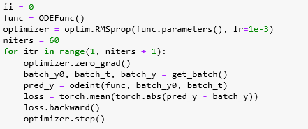
To run Tune on the model you need to wrap it in a function that will encapsulate the model with instances of the configuration. The wrapped model executes a standard (in this case torch) training loop followed by a validation loop which computes an average loss and accuracy for that set of parameters.


One of the most interesting part of Tune is how they schedule the training-validation tasks to search the space to give the optimal results. The scheduler choices include HyperBand, Population Based Training and more. The one we use here is Asynchronous Successive Halving Algorithm (ASHA) (Li, et.al. “[1810.05934v5] A System for Massively Parallel Hyperparameter Tuning (arxiv.org)” ) which, as the name suggests, implements a halving scheme that rejects regions that do not show promise and uses a type of genetic algorithm to create promising new avenues. We tell the scheduler we want to minimize a the loss function and invoke that with the tune.run() operator as follows.

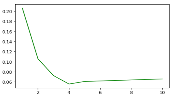
We provide the complete code in a Jupyter notebook. The model we are training to solve is the classic and trivial Iris classification, so our small Neural network converges rapidly and Tune gives the results

Note that the test set accuracy was measured after ray completed by loading the model from checkpoint that Tune saved (see the Notebook for details)
Final Thoughts
There are many aspects of Ray that we have not discussed here. One major omission is the way Ray deploys and manages clusters. You can build a small cluster on AWS with a one command line. Launching applications from the head node allows Ray to autoscale the cluster by adding new nodes if the computation demands more resources and then releases those node if no longer needed.
In the paragraphs above we focused on two Ray capabilities that were somewhat unique. Ray’s actor model in which actors can persist in the cluster beyond the lifetime of the program that created them. The second contribution from Ray that we found exciting was Tune. A use case that is more impressive that our little Iris demo is the use of Tune with hugging face’s Bert model. See their blog.