Chapter 10.4 of ‘Cloud Computing for Science and Engineering” described the theory and construction of Recurrent Neural Networks for natural language processing. In the three years since the book’s publication the field of language modeling has undergone a substantial revolution. Forget RNNs. Transformers are now in charge, so this report is an update of that part of the chapter.
The original RNNs were not very good at capturing the context of very long passages. A technique was developed, called ‘attention’ that was an add-on to the RNNs to help them with this problem. In a landmark paper, “Attention is all you need”, Viswani, et. al. showed that the recurrence part was not really needed. This supplement will describe the basic transformer architecture and look at three examples. The first is called BERT and it was the transformer that changed the field of natural language processing. We will briefly describe its architecture and demonstrate how to use it with an optimized version called RoBERTa. Finally we will move onto a more recent transformer called XLNet that has drawn a lot of interest.
There are dozens of blog posts and articles on-line that describe transformers and the original papers do a great job describing the mechanical details. The challenging part is understanding how the details of the network design capture the networks ability to model the probability distributions associated with natural language. What do I mean by that? Consider the sentence “He decided to walk across the lake.” A native English speaker would be troubled by that and, perhaps suggest that an error occurred and the sentence should have been to be “He decided to walk across the lane.” There is nothing grammatically wrong with the first sentence. It just does not feel right. It is beyond normal in the internal language model we use for comprehension.
We can also consider ‘fill in the blank’ test to see how we draw on reasonable expectations of how words fit into context. For example, consider these three sentences.
- “Because she was a good swimmer, she decided to <mask> across the <mask>”
- “He went to the farmer’s <mask> and <mask> a bunch of green <mask>.”
- “Whenever <mask> go to the whiskey <mask>, <mask> have a lot of <mask>”
In sentence 1 the masked pair could have been “walked”, “road”, but context “swam”, “lake” is more natural because, in context, she is a swimmer. For sentence 2, the masked triple could be “home”, ”ate”, ”cars”, but “market”, “purchased”, “beans” feels better. We leave it to your imagination to decide what fits in sentence 3.
A masked language model is one that can input words in sentences like those above and any masked word is replaced by something that, with reasonably high probability, fits in the context of the sentence. Before launching into experiments with masked language modes let’s briefly look at the architecture of transformers as described in the original Viswani paper.
Bert and the Transformer Architecture
A transformer has two major components: an Encoder and a Decoder. The Transformer has an implicit model of language in that it has learned a probability distribution that is associated with “meaningful” sentences in the language. The encoder is a non-linear function that maps an input text object into an object in high dimension real space that is somewhat “near” very similar sentences. To do this, Transformers have a special tokenizer that can convert text into token lists, where each token is an integer index into a vocabulary list for that transformer. More specifically let s be a string, then let In_tokens = Tokenizer.encode(s) and n = length(in_tokens). The Encoder has an embedding function
Encoder.input_embedding: ZM -> Rk
Where M is the size of the model vocabulary and k is the model-specific dimension of the embedding space. Hence the representation of the entire string is n vectors of dimension k (or vector of dimension Rk*n ). There is a now famous diagram that illustrates the architecture of the transformer.
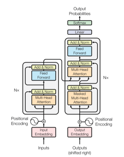
Figure 1. The transformer model (from “Attention is all you need”, Viswani, et. al.)
The full encoder is the vertical stack on the left. So far, we have only described the Input Embeddings. Ignoring (for now) the Positional Encoding, note that our Rk*n input is fed to a stack of “N” blocks, each of which consists of a Mult-Head Attention and a Feed forward network, each of which generate a new Rk*n vector output. The Multi-Head Attention block consists of a parallel collection of scaled dot product blocks as illustrated in Figure 2.
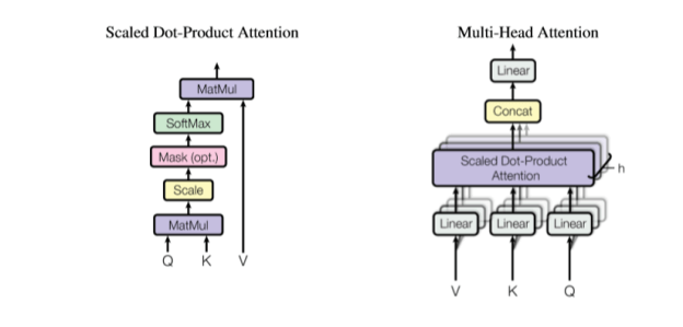
Figure 2. Multi-Head Attention and Scaled-Dot-Product Attention (again from Viswani et. al.)
The basic Attention part is the critical component. It is a function of three tensors. Q is called the query tensor and it is of dimension nxt for some t and K is called a key tensor and it is of the same dimension. The keys are “associated” with values in the vector V which is of size nxk. The attention function is then
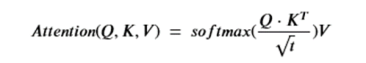
Note that Q*KT is of size nxn. The softmax is applied to each row of the product (after normalizing by the square root of t), so the final result is nxn time nxk which is size nxk. The way to think of this function is that each t dimensional query vector is being dot-product compared to each key vector. If those two vectors are nearly orthogonal then the dot-product is small and the corresponding row on the result of then attention function will be small. Here is the motivational concept. Let’s suppose the queries are associated with words in a sentence and we want to see what other words in the sentence are most related. The other words are keys. So if the sentence is “John got in his car then he went to the store”, then we would expect a strong link between “John”, “his” and “he” as illustrated below.
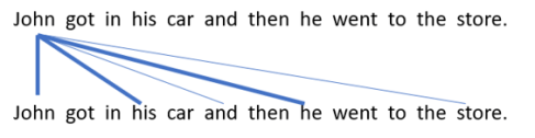
Figure 3. Dark lines indicate where we expect the attention between words to be the strongest. (Apologies to those who feel the reference to gendered pronouns is bad.)
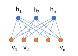
Now to explain the Multi-Headed Attention. We are going to replicate the scaled dot-product attention network h times where h is a divisor of k and we set t = k/h. Our embedded sentence is of dimension nxk, so to create the Q, K and V vectors we have to project these into vectors of size nxt (for Q and K) and nxk for V. These projections are the linear transformations in Figure 2. Also we now have h outputs of size nxk. We concatenate those outputs and use a final linear map to project it back to a single nxk vector.
The idea of multiple heads is to allow different heads to attend to different subspaces of attention. It also slightly reduces the computational complexity of the attention convergence computation. However, there is some question as to whether multiple heads helps that much (see “Are Sixteen Heads Really Better than One?” by Michel, Levy and Neubig.)
The final critical component of the network is the feed forward block. This is a basic two-level network with one hidden layer. Notice that this does not involve token-to-token analysis; that was the job of the attention blocks. Hence the network can process the tokens independently, so its internal structure is independent of the token stream length.
There are other components of the Transformer including the add & norm steps and the Decoder. The Decoder half has the same basic components as the Encoder, and it is the part that is critical for building language translation systems but we will not address that task here. (A good discussion of the Decoder is given in “Dissecting BERT Appendix: The Decoder”, a Medium post by Miguel Romero Calvo.)
There are several other ways to train a model like this and one is to turn it into a masked language model. To do this we wrap the basic Encoder with a “Masked Language Model Head”. To explain this, we need to get into a few details related to the experiments we will show.
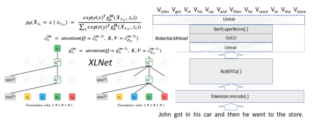
The original Transformer version, BERT (Bidirectional Encoder Representations from Transformers) was developed by Google, but we will use the more optimized version called RoBERTa (from Facebook and the University of Washington), which was released together with the paper a Robustly Optimized BERT Pretraining Approach by Yinhan Liu, Myle Ott, Naman Goyal, Jingfei Du, Mandar Joshi, Danqi Chen, Omer Levy, Mike Lewis, Luke Zettlemoyer, Veselin Stoyanov. (RoBERTa was trained with mixed precision floating point arithmetic on DGX-1 machines, each with 8 × 32GB Nvidia V100 GPUs interconnected by Infiniband.) The Roberta Masked language model is shown in Figure 4 below. The RobertaMaskedLanguage model is composed of a Language Model head on top of the base language model.
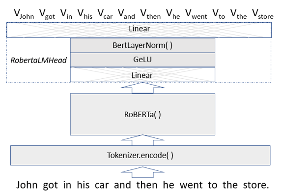
Figure 4. Vword = a vector of probabilities indexed by words in the vocabulary.
The LM head consists of a linear transformation normalized with GeLU (Gaussian Error Linear Unit) activation and then again with the a LayerNorm function ( (x – x.mean)/|x-x.mean| ) followed by a linear transformation mapping the result back into a list of vectors of probabilities each of which has length equal to the size of the vocabular. The length of the vector list is the number of tokens in the original input. If the transformer is doing its job, the vector of probabilities associated with a given work-token has a maximum at the index of that word (or a better one) in the vocabulary. (The Masked Language Header also returns cross entropy loss of the predicted values from the input string, but we will not use that here.)
Demo Time!
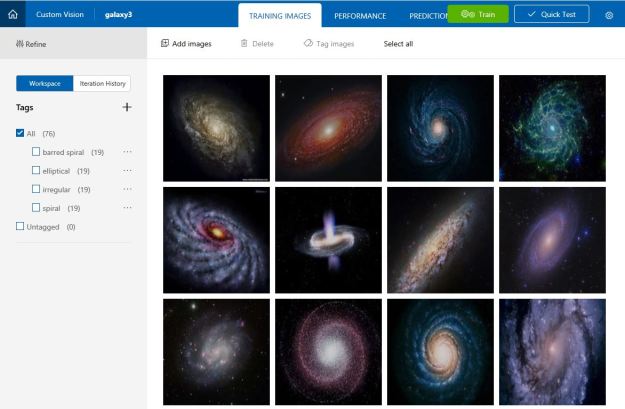
To illustrate the behavior of RoBERTa language model can load an instance as follows. We can use the PyTorch-Transformers by HuggingFace Team who have provided excellent implementations of many of the examples in the Transformer family.
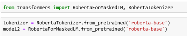
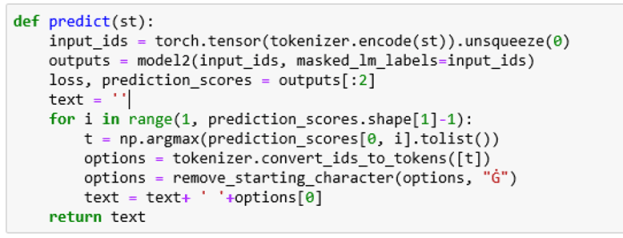
Roberta-base has 12-layer, 768-hidden, 12-heads and 125M parameters. To use the model, one need only convert a text string to a tensor of input tokens, feed that to the model and pull out the list of prediction scores (which is returned as a tensor with shape string-length by vocabulary size). Taking the largest prediction as the likely correct word and converting that back to a token ( and removing an internally added character) yields the result. In code this is:
To illustrate this on a simple sentence, we will use one that is not grammatically correct and see what the model comes up with.
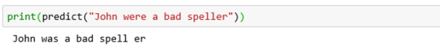
Notice two things. The model split the word speller into a root and suffix. But the model generated a new sentence that was closer to what the probability distribution said a current sentence should look like. In this case that was a change from “were” to “was”.
To illustrate its use as a masked model we can substitute words in the text with a <mask> to see how the model replaces the masks.

In this case it matched the pronoun “she” and inferred that “swim” and “lake” was a good choice.
Changing the context slightly we have

Taking our first example from the list of three above,

And finally, our third sample sentence

The source notebook for this example is in the GitHub archive. Load it and try it out yourself.
XLNet and sentence generation.
Another important point we neglected to discuss in the discussion of BERT, involves the position of tokens in the input. The Attention operation compares each work in the string with each other word “in parallel”, however the order of words in the string matters if we want to understand its meaning. Hence, it is necessary to tag each token with position information. The way this is done is to create an additional value (based on a clever use of sine waves of different frequency … the details are not important here) to encode position in the string. These values are literally added to the embedding values before being sent to the Attention function. This is a detail we do not see when we invokee the RobertaForMaskedLM model. It is handled internally. (You can see it referenced in Figure 1.)
BERT is an autoencoding (AE) language model: it is trained to recover masked tokens in its input. XLNet is a newer Transformer language model that is showing better performance than BERT or RoBERTa on many test cases. BERT derives its power to predict a token at sequence position t from the fact that it looks at both the elements larger than t and smaller than t. But BERT has one subtle weakness. Because the it is trying to predict masked tokens ‘in parallel’, that does not mean that it will predict them consistently. For example, “”he went to the <mask> <mask> and purchased lots of postage stamps.” gives BERT a hard time. It tries to replace the pair of masks with “store store”, instead of “post office”. (Replacing postage stamps with vegetables and it guesses “grocery store”)
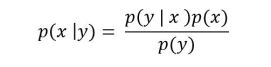
An autoregressive model, like XLNet, operates differently. Given a string of word-tokens X = [x1, x2, … , xt], an autoregressive language model will try compute a sequence of conditional probabilities to compute p(X)
![]()
The problem with this is that is that if we are going from the left to right, we miss the context for words that have important information that are to the right. BERT avoids this by doing all words in parallel. Developed by Yang, Dai, Yang, Carbonell, Sakakhutdinov and Le from CMU and Google, XLNet is referred to as a generalized autoregressive (AR) language model. Rather than do the predictions from the left (x1) to right (xT ), XLNet uses all permutations of the tokens to do the computation.
The following is very abstract and a bit confusing, so feel free to skip this next part and go to the fun demos that follow.
Let ZT be the set of all possible permutations of the length-T index sequence [1, 2 ,… ,T]. Let z be a permutation in ZT. The notation zt refers to the tth element in the permutation. Similarly, z<t refers to the t-1 elements of the permutation that precede it. We can apply the same conditional probability sequence stated above to elements in the permutation order to compute the conditional probability
![]()
The key idea is that if we compute the probabilities for the correct word at each position in the string using every permutation of the words in the string then all contexts for the word in that position can be considered. For example the sentence “He is tall.” Looking at the permutations
He is tall –
tall He is +
is tall He +
tall is He +
is He tall –
He tall is –
If we compute the probabilities from left to right of each of these permutations we see that the permutations marked with a + have the word “tall” before “He”, so in calculating the conditional probabilities p(“He” | … ) we see the word “tall” is encountered in that computation. If the sentence had been “He is talls”, these conditional probabilities would have been lower and the result would have been lower.
The XLNet designers decided to train a network that would use this principle as a goal and optimize the network parameters (theta) to find
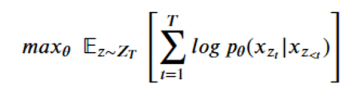
The result is a sequence of M query operators g that are defined by the model parameters, such that for each permutation the conditional probability can expressed in a softmax form as
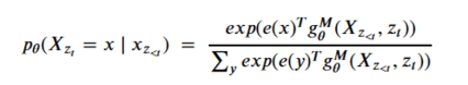
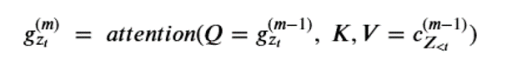
That is, for position zt in a permutation , g is a function of the elements that precede it and on the position itself (and not the value at that position.) Computing the sequence of query operators g we need to use what the authors call a two stream recurrence. One sequence is called the content stream and it is computed as

Notice that the content at the next level up depends on the position zt as well as the value xzt . (Notice the <= in the KV pair. While this may seem like an obscure point, it is important that g depend only on the position in the permutation and not the value there because we are trying to compute the condition probability of that value!) We now define the query operator g by
For each permutation we initialized the recurrences with
![]()
Where w is a learned parameter and, in the case of strings longer than 512 words, the previous 512 blocks.
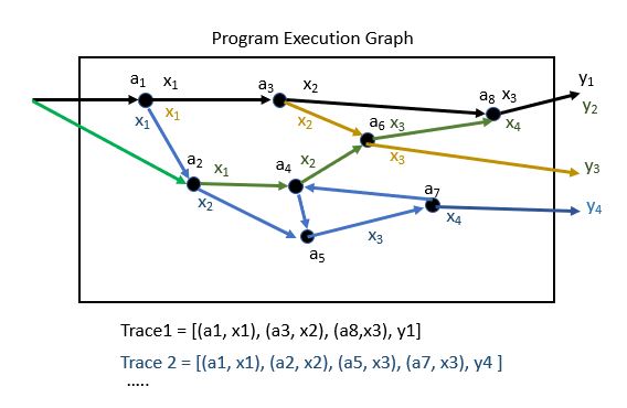
If these recurrences look too abstract, here is how they look in a (simplified) version of the attention stack.
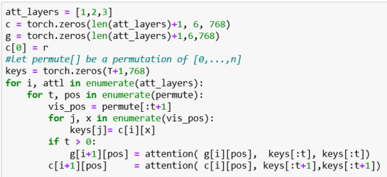
What this fails to show is how values are averaged over multiple different permutations.
Demo Time Again!
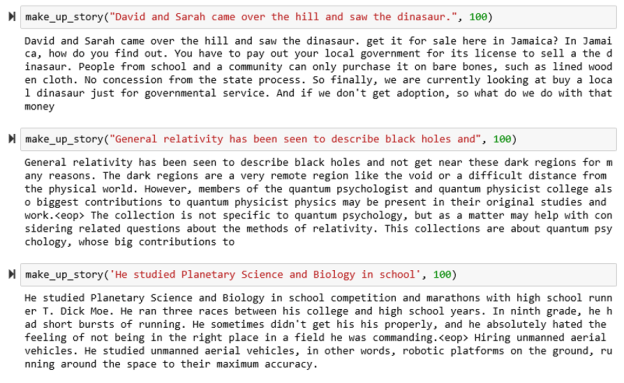
This demo will be to use XLNet to generate stories. The way this works is that we will start with a sentence fragment and we will add an extra token at the end and get XLNet to predict the next word. We then add that word to the end of the sentence and repeat the process.
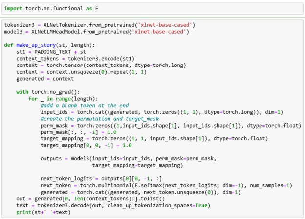
We have cast this process as a function which takes a string and an integer to indicate the length of the string we want to make. XLNet likes to have a long string to start, so we have added a paragraph of PADDING_TEXT at the beginning.
To force the model to generate the new last word, we do a bit of black magic. We need to generate a permutation mask and a target mask. We are using the excellent HuggingFaces library of Transformer implementations. The API for their XLNetHeadModel can be found here. We first add a blank token to the end of the list of ids (this is just a 0). If the length of the input_ids is m, then the perm_mask is of dimension 1xmxm and all zeros except the last column which is all ones. The target mapping is 1x1xm is all zeros except the last element which is a one. The target mask tells us which outputs we want and, in this case, it is only the last element.
The output is a list whose first element is a tensor of dimension 1x1x3200. This is the vector of token logit values for each word in the 3200 word dictionary. To select the word, draw a sample from a multinomial distribution based on softmax of the logit vector. Because of this random draw the results are never the same twice when we run the function. Below are some samples.
The source notebook for this demo is xlnet-story-generator.ipynb in github.
Document classification
Document classification with Transformers require you to add a doc classifier head to the basic model. In the case of both Bert and XLNet the 0th position of the last hidden state can be considered as a summary of the document as a vector of size 765 and a Tanh activation function is applied to that.
The Classifier basically consists of an additional linear layer of size 765xq where q is the number of classes as shown in figure 5 below.
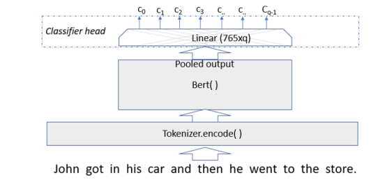
Figure 5. Document classifier uses pooled output from Bert (or XLNet) as input to an additional linear layer to do get final classifier values.
In the experiments that follow we will use Thilina Rajapakse’s Simple transformers library which wraps the standard HuggingFaces library in a way that make the entire process very simple.
Demo—Classifying Scientific Abstracts
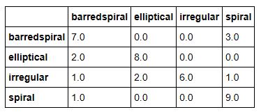
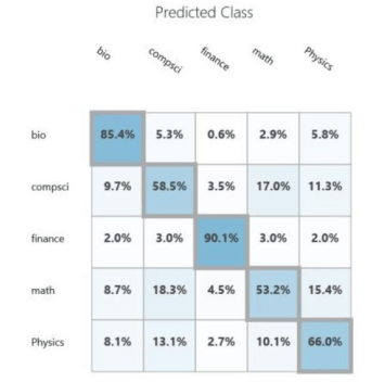
The documents we are going to classify are abstracts of papers from Cornel’s ArXIV. The collection we are going to use is small (7100 paragraphs). ArXIV is a collection of papers that are submitted by scientists and are self-classified into one or more of several dozen categories. In our case there are papers from 138 subtopics and we have grouped them into 5 broad categories: Math, Computer Science, Biology, Physics and Finance. These categories are not uniformly represented and to make things very complicated there are many papers that could be classified in several of these broad groups. This is not surprising. Science is now very multidisciplinary. It is not unusual to find a mathematics paper about computational biology that uses techniques from computer science. Or a physics paper that uses neural networks with an application to finance. We first experimented with this data collection in Nov. of 2015. We used a very early version of the Azure ML Studio. The confusion matrix for the result is shown below. As you can see, it is not very impressive.
We looked at this problem again in Nov of 2017, but this time we used document analysis with the package genism.
And once again the results were underwhelming. If want to classify these documents with a Transformer, we must first train the top layer to fit our data. These two lines are sufficient to create the model and train it.
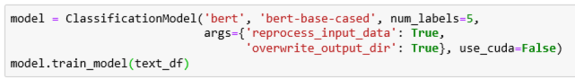
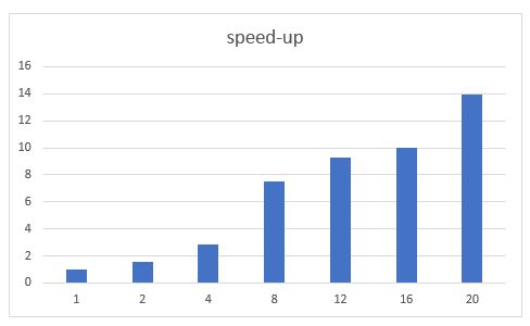
The input to the train function is a Pandas data frame with one column the text of the abstract and the second column the classification into one of our five categories. The training on an Intel Core-7 takes about 20 minutes. Creating and training the same model with XLNet takes about 30 minutes.
We trained the model with 4500 of the abstracts and evaluated it with 2600 of the remaining abstracts. To do the evaluation you use

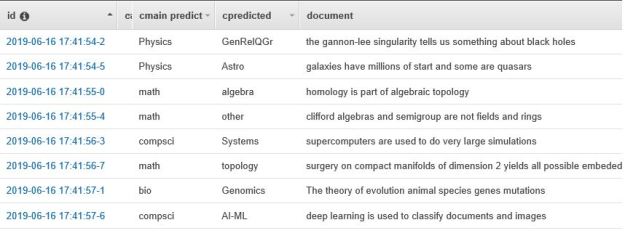
Result is a 2600×5 tensor where each row a vector of length 5 that is the softmax of the model predictions. Wrong predictions is a tensor that described where the model failed. This information is very interesting and it illustrates the types of “interdisciplinary” confusion that can arise. Here are three examples of failures.
A Math paper predicted to be Computer Science.
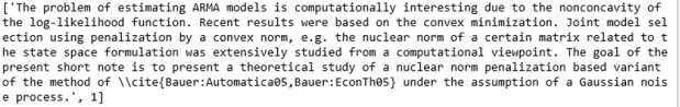
A Physics paper predicted to be Math.
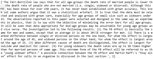
Finally a Finance paper predicted to be Physics
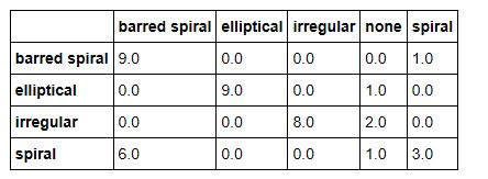
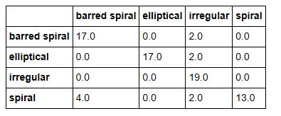
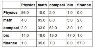
It is the last sentence that is the clue that this is finance related. We now can use the results output to compute the confusion matrix. Here are the results for BART and XLNet.
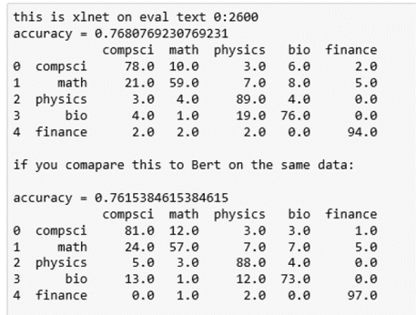
As can be seen the XLNet results were, on average, slightly more accurate and both methods were superior to the older approaches described above.
The interesting data here is the frequency with which Math papers are labeled as Computer Science. This is largely due to the fact that the major of papers about neural networks are in the computer science category, but there are also many mathematicians that are looking at this topic.
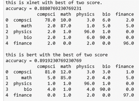
Because we have the softmax ‘probabilities’ for the classification of each document, we can ask about the 2nd most likely choice and compute a “best-of-2” score for each paper. In other words, an X paper is classified as X if one of the two top predictions is an X. The results are shown below. As you can see, it resolves the math-cs confusion as well as bio-physics.
The data and notebook for this demo are available in GitHub.
Final Thoughts
The experiments on document classification are simple illustrations. The Transformer scientific literature has a host of tests to which all of these methods have been subjected. The careful reader will notice that in the examples we have illustrated above, we only used the smallest of the available language models of each type. This was to allow our Notebooks to run in a relatively standard laptop. Of course XLNet is not the last word in Transformers. Some of the new models are huge. For example Microsoft had just announced Turing-NLG, with 17 billion parameters.
One of goals of Turing-NLG and many other Transformer models is to improve performance around some important tasks we did not discuss above. For example, question answering and document summarization. These are very important examples. For example, the Stanford Question Answering Dataset (SQuAD 2.0) is often cited. Another application of Transformers is uncovering the structure of language expressions. John Hewitt has done some interesting experiments along these lines in Finding Syntax with Structural Probes, In Oct of 2019 we posted an article “A ‘Chatbot’ for Scientific Research: Part 2 – AI, Knowledge Graphs and BERT” where we discussed the role Transformers are playing in only search and the role they will play in smart digital assistants. We concluded there that it was necessary to extend the analysis from sentences and paragraphs to incorporate additional information from knowledge graphs. Chen Zhao et.al. from Microsoft consider aspects of this problem in the paper Transformer-XH: Multi-Evidence Reasoning with Extra Hop Attention. We are excited by the progress that has been made in this area and we are convinced that many problems remain to be solved.


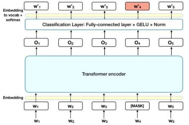 Figure 5. Bert training of the encoder based on masking random words for the loss function. This figure taken from “BERT – State of the Art Language Model for NLP” by Rani Horev in
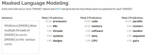


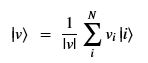


 Using this basis, any qubit |Ψ> can be described as a linear combination (called a superposition) of these basis vectors
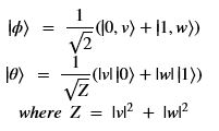
 where α and β are complex numbers whose square norms add up to 1. Because they are complex this means the real dimension of the space is 4 but then the vector is projected to complex projective space so that two qubit representatives |Ψ> and |г> are the same qubit if there is a complex number c such that
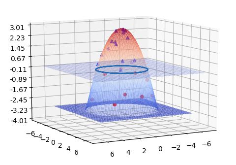
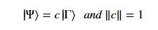 A slightly less algebraic representation is to see the qubit |Ψ> as projected onto the sphere shown on the right
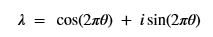
  where |Ψ> is defined by two angles where
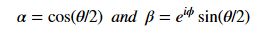


 This braded structure is a topological constraints that is a global property and therefor very robust. If you can make a qubit from this property it would impervious to minor noise.