Category Archives: machine learning

Fun with Recurrent Neural Nets: One More Dive into CNTK and TensorFlow

In a previous article I set about comparing Microsoft’s Computational Network Took Kit for deep neural nets to Google’s TensorFlow.  I concluded that piece with a deep dive into how recurrent neural nets (RNNs) were represented in each system.   I specifically went after the type of RNNs known by the strange name of Long Short-Term Memory (LSTM) networks.   I wanted to learn a bit more about how these systems worked.  I decided to treat them like laboratory specimens so that I could poke and prod them to see what I could learn and what I could get them to do.  This article is essentially my lab notebook.  Warning:  With the exception of a bit toward the end, this is not technically very deep.   In fact, I did not discover anything that has not been extensively reported on elsewhere.   But I learned a lot and had some fun.   Perhaps it will be of interest to students just starting to learn about this subject.   Before I get to far into this, I would like to mention that I recently discovered an excellent series of tutorials on RNNs by Denny Britz that are definitely worth reading.

CNTK’s LSTM and Hallucinating Bloomberg Financial News

One of the many good examples in CNTK is language modeling exercise in Examples/Text/PennTreebank.   The documentation for this one is a bit sparse and the example is really just of a demo for how easy it is to use their “Simple Network Builder” to define a LSTM network and train it with stochastic gradient decent on data from the Penn Treebank Project.   One command starts the learning:

cntk configFile=../Config/rnn.cntk

Doing so trains the network, tests it and saves the model.  However, to see the model data in an easily readable form you need a trivial addition to the configfile: you need to add the following dumpnode command to put a dump file a directory of your choosing.

dumpnode=[
    action = "dumpnode"
    modelPath = "$ModelDir$/rnn.dnn"
    outputFile = "$OutputDir$/modeltext/dump"
]

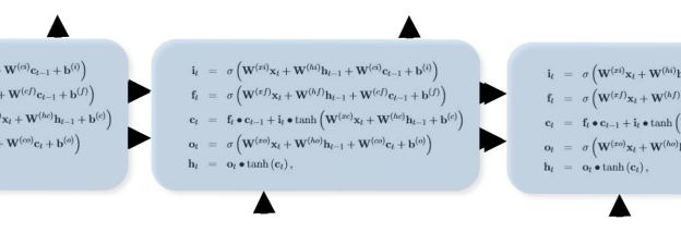
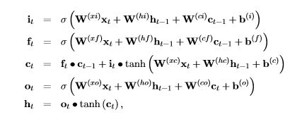
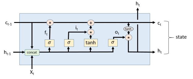
This creates a big text file with all the trained data.   To experiment with the trained model, I decided to load it into a python notebook and rebuild the LSTM network from the defining equations.  From the CNTK book those equations are

lstm_eqn

I was pleased to see that the dumped model text had the same W and b tensors names as in the equations, so my job was relatively easy.    I extracted each of the tensors and saved them into a file (I will make these available in Github).   The python code for the LSTM based on the equations above is below.

def rnn(word, old_h, old_c):
      Xvec = getvec(word, E)

      i = Sigmoid(np.matmul(WXI, Xvec) + 
                  np.matmul(WHI, old_h) + WCI*old_c + bI)
      f = Sigmoid(np.matmul(WXF, Xvec) + 
                  np.matmul(WHF, old_h) + WCF*old_c + bF)
      
      c = f*old_c + i*(np.tanh(np.matmul(WXC, Xvec) + 
                               np.matmul(WHC, old_h) + bC))
      
      o = Sigmoid(np.matmul(WXO, Xvec)+ 
                  np.matmul(WHO, old_h)+ (WCO * c)+ bO)
      
      h = o * np.tanh(c)
      
      #extract ordered list of five best possible next words
      q = h.copy()
      q.shape = (1, 200)
      output = np.matmul(q, W2)
      outlist = getwordsfromoutput(output)
      return h, c, outlist

As you can see, this is almost a literal translation of the equations.    The only different is that this has as input a text string for the input word.  However the input to the equations is a vector encoding of the word.  The model generates the encoding matrix E which has the nice property that the ith column of matrix corresponds to the word in the ith position in the vocabulary list.  The function getvec(word, E) takes the embedding tensor E, and looks up the position of the word  in the vocabulary list and returns the column vector of E that corresponds to that word.   The output of one pass through the LSTM cell is the vector h.  This is a compact representation of the words likely to follow the input text to this point.  To convert this back into “vocabulary” space we multiply it by another trained vector W2.  The size of our vocabulary is 10000 and the vector output is that length.  The ith element of output represents the relative likelihood that that ith word is next word to follow the input so far.  Getwordsfromoutput simply returns the top 5 candidate words in order of likelihood.

Before going further, it is worth looking closer at the properties of the word embedding matrices E and W2.   There is a fascinating paper by  Mikolov, Yih and Zweig entitled “Linguistic Regularities in Continuous Space Word Representations” where they suggest that the embedding space for word has several interesting properties.   I decided to investigate that.   Their point is that words that are similar in a linguistic sense will be nearby in the embedding space.   For example, present tense verbs should be near other present tense verbs and singular nouns should be near each other, etc.   I decided to try that.  However, there are two embedding mappings.  One is based on the tensor E and the other based on the W2 tensor.   E has dimension 150 by 10000 and W2 is 200 by 10000.  The difference in dimensionality are because of arbitrary decisions made in defining the hidden layers in the network.  But both represent word imbeddings.  I experimented with both.  I wrote a function getnear(word, M) which takes a word and looks for the 5 most nearby words in the space where M is transpose of either E or W2. (I used cosine distance as the metric.) Verb tense locality and noun plurals worked best in the W2 space as illustrated below.

rnn-embedding

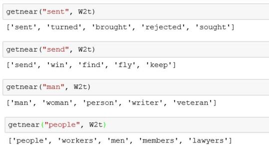
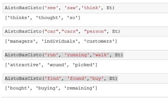
These are only illustrations.  For a deeper statistical analysis look at the Mikolov paper.   A more interesting conjecture from their study was that there may be some linearity in these embedding that might allow one to try simple analogies of the form “A is to B, as C is to __”.   Their idea is that if a, b and c are the vector embeddings of the words A, B and C, then the embedding of “__” may be computed as d = c + (b-a).  So I wrote a little function AistoBasCisto(A, B, C) that does this computation.   In the results I had to delete A, B and C from the candidate answers because they came up often as nearby.   In this case my results were less encouraging.  It worked better with the E space than with W2.   For example, for E we have

rnn-analogy1

And for the W2 space the results looked like

rnn-analogy2

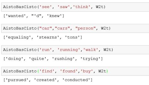
As you can see the “run running walk __” example failed with E but was close, but still incorrect, with W2.

You may wonder why these particular words came up.  The data we used to train the system came from a small subset of the Penn TreeBank collection as provided in the CNTK package.   It is heavily dominated by financial news items.    This explains why the plural of person could be managers or customers.   A larger vocabulary and data collection would be needed to truly test the analogy by linearity conjecture.

Now on to hallucinating the financial news.

Now to test the LSTM as a truly recurrent network.   We provide the network with a starting word and let it suggest the next word.  And then we repeat this process constructing a “sentence”.  In the code below we randomly pick one of the top three suggest by the network as the next word.

c = np.zeros(shape = (200, 1))
h = np.zeros(shape = (200, 1))
output = np.zeros(shape = (10000, 1))
word = 'my'
sentence= word 
for _ in range(40):
    h, c, outlist = rnn(word, h, c)
    word = outlist[randint(0,3)]
    sentence = sentence + " " +word
print sentence+"."

In this case we start with the word “my” and let it generate a 40 word sentence.  The output is

my new rules which would create an interest position here unless there should prove   signs of such things too quickly although the market could be done better toward paying further volatility where it would pay cash around again if everybody can.

This is a great example of hallucinating financial news. Let’s try it again starting with the word “president”.

president michael de brown wrote himself against democratic union law which represents an emergency relief agreement during a new york state district or early tuesday before july after a federal government agency created early losses without mr. krenz or perhaps.

Now with the word “the”.

the company reported third-quarter results reflecting a number compared between N barrels including pretax operating loss from a month following fiscal month ending july earlier compared slightly higher while six-month cds increased sharply tuesday after an after-tax loss reflecting a strong.

The “sentences” end rather abruptly because of the 40 word limit I set.  If you let it go it will run on until the state vector for the sentence seems to break down.     Try this yourself.  To make it easy to play with this example, I have put the code in GitHub.  The trained model text files are in OneDrive and is a zipped file of about 50MB.

There are many more excellent and fun examples.  Andrej Karpathy has a great blog article showing how RNNs can mimic Shakespeare, or Latex science articles and many more.

TensorFlow’s seq2seq French Lesson.

One of the most interesting examples in the TensorFlow tutorials is an English to French translator.  As with the CNTK example it was trivial to start the translator learning following the instructions in the tutorial.   After letting this run for about a week, I wanted to see how well it would do.     As with the CNTK example, I created a Jupyter IPython notebook and loaded the trained model.   I will explain how that was done in more detail below but, for now, I will show how we can invoke it to test its translation ability.    This particular trained model was not very big and with a relatively small data set, so I didn’t expect much.    In fact, as you will see, to a French speaker it is a disaster.   On the other hand, it learned more French in a week of training that I did in three semesters of French in college.   (For full disclosure, this was my weakest subject in college and my grade was a hard-fought “C” each semester.)

The code below demonstrates how the model is invoked.   First you have to tokenize the input sentence.  The algorithm uses a system of buckets of fixed sizes to make the training more efficient.  You next find the smallest bucket that can contain your sentence and convert this to the input vector list needed by the model.   The step function takes a Tensorflow session, the input vector list and a null list of decoder inputs (to be explained later) and generates a list of vectors as outputs.  Each vector represents the likelihood that individual vocabulary words are the correct word at that point in the translated sentence.   We pick the most likely and print the sentence.

sentence = " I am not the president of France. "

token_ids = data_utils.sentence_to_token_ids(sentence, en_vocab)
      # Which bucket does it belong to?
bucket_id = min([b for b in xrange(len(_buckets))
                 if _buckets[b][0] > len(token_ids)])
      # Get a 1-element batch to feed the sentence to the model.
encoder_inputs, decoder_inputs, target_weights = 
    model.get_batch({bucket_id: [(token_ids, [])]}, bucket_id)

_, _, output_logits = model.step(sess, encoder_inputs, decoder_inputs, 
                                 target_weights, bucket_id, True)
		  
outputs = [int(np.argmax(logit, axis=1)) for logit in output_logits]
print(" ".join([rev_fr_vocab[output] for output in outputs]))

Je ne suis pas le président de la France .

This example is not too bad.  However, if I ask

“In which city does the president of France live?”

I get

“Dans quelle ville le président de la France ?”.

This is not exactly correct.    If I feed this into Google translate and ask what this means in English I get “In which city the President of France?”.   If I give it this one,

What is the name of a good restaurant?

The system responds with

Quel est le nom d’une bonne bonne bonne ?”

Which translates back to “What is the name of a good good good?”.  Probably not very helpful on the streets of Paris.   It turns out restaurant is not in the tiny training vocabulary used here.   Finally, given this sentence

” The article stated that the President of the United States is here today. “

The translator returned

Le paragraphe a indiqué que le président des États-Unis est aujourd ‘ hui aujourd ‘ hui .”

The end of this reply is “is today today”.    As I said, this is still much better than I could do with my college French.   However, as you can see from the previous two examples, our little translator runs out of gas at the end of sentences and tends to repeat itself.   You should try this yourself.   I have put the notebook file in github or you can execute these directly from the Tensorflow python code.   All you need to do is train the model from TensorFlow and run the notebook with the path to the model output directory.

While loading and using the trained model was easy and fun, understanding the seq2seq model used in this example takes a bit of work.   So this part of this article will get a bit more technical.

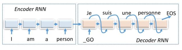
The TensorFlow translate program is based on a sequence-to-sequence model constructed from more primitive recurrent neural nets.   By sequence-to-sequence we mean a network that takes a sequence as input and produces a sequence as output.   It consists of two parts: an “encoder RNN” and a “decoder RNN” as shown in Figure 1 below.

seq2seq

Figure 1.   A sequence-to-sequence RNN English to French translator with the encoder and decoder unrolled to show the flow of messages.

In this figure the RNNs are “unrolled” to show the flow of messages.  The state vector at the end of the encoder is a vector embedding of the input sentence.   This state vector is used to start the decoder along with a “GO” token.  The diagram shows the network after it has been trained.   During training the inputs to the decoder are the French version of the English sentences.   I won’t talk about the training here because is enough to try to understand how this works.  Before I go any further I want to point you to some important papers.  Sutskever, Vinyals and Le published an early important paper on sequence to sequence models that is worth reading.

To understand how it is built the network we need to dig into the code a bit. The building blocks are a set of classes of base type RNNCell with specializations

  1. BasicRNNCell
  2. GRUCell
  3. BasicLSTMCell
  4. LSTMCell
  5. OutputProjectionWrapper
  6. InputProjectionWrapper
  7. EmbeddingWrapper
  8. MultiRNNCell

The ones we will see used here are GRUCell, MultiRNNCell and EmbeddingWrapper.   We discussed LSTMCell in our previous article but we need to look at GRUCell here because that is the one used in the example.   The GRUCell is a “Gated Recurrent Unit” invented by Cho et. al.  in “Learning Phrase Representations using RNN Encoder–Decoder for Statistical Machine Translation”.  The “gated” phrase comes from the way the output is defined as coming mostly from the previous state or from a combination with the new input.   The diagram below tries to explain this a bit better.

gru-pic

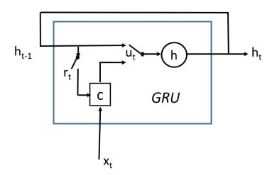
Figure 2.   GRU wiring diagram

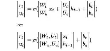
It also helps to see it in terms of the defining equations.

gru-eq1

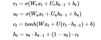
The quantity ut  is a gate vector.  Recall the sigmoid function switches sharply between one and zero.  So when ut is one then h is just a copy of the old h and we are ignoring the input x it is based on the value ct.   The gate rt is determines how much of the old state goes into defining the value of ct.   To understand how this is encoded in TensorFlow you need to understand the function.

linear(args, output_size, bias, bias_start=0.0, scope=None)

where args is a list of tensors each of size batch x n .   Linear computes sum_i(args[i] * W[i]) + bias where W is a list of matrix variables of size n x outputsize and bias is a variable of size outputsize.   In the equations above we have represented linear algebra as a matrix times a column vector.   Tensorflow uses the transpose notation:   row vector on the left times the transpose of the matrix.   So in linear the args are a list of row vectors.   Where is the matrix W and offset b?  This is fetched from memory based on the variable current scope, because W and b are variable tensors that are learned values.   If you look at the first two equations above, you will see they are almost identical.   In fact, we can write them as

gru-eq2

If you transpose the last one from column form into row form you can now compute both with one invocation of the linear function.   The code for the GRUCell is below.   As you can see they have encoded one pass through the GRU cell with only two matrix vector multiplies.   You can also see that the way the variable scope is used to pick out the W’s for the gates and the W for the state/output.  Another point to remember that an invocation of the “__call__ function operator does not cause the tensor to execute the operation, rather it builds the graph.

class GRUCell(RNNCell):
  def __init__(self, num_units):
    self._num_units = num_units
   ... stuff deleted ....
  def __call__(self, inputs, state, scope=None):
    with vs.variable_scope(scope or type(self).__name__):  
      with vs.variable_scope("Gates"):  # Reset gate and update gate.
        # We start with bias of 1.0 to not reset and not udpate.
        r, u = array_ops.split(1, 2, linear([inputs, state],  
                               2 * self._num_units, True, 1.0))
        r, u = sigmoid(r), sigmoid(u)
      with vs.variable_scope("Candidate"):
        c = tanh(linear([inputs, r * state], self._num_units, True))
      new_h = u * state + (1 - u) * c
    return new_h, new_h

The top level class we invoke for building our model is seq2seqModel.    When we create an instance of this class it sets in motion a set of flowgraph building steps.  I am going to skip over a lot of stuff and try to give you the big picture.  The first graph building step in the initialization of an instance of this object is

# Create the internal multi-layer cell for our RNN.
    single_cell = rnn_cell.GRUCell(size)
     …
    if num_layers > 1:
      cell = rnn_cell.MultiRNNCell([single_cell] * num_layers)

As you can see we are creating a GRU cell graph generator instance and making a list of num_layers of this object and passing that to the constructor for MultiRNNCell.   In our case, num_layers has been set to 2.   MultiRNNCell is pretty easy to understand.   It builds a graph consisting of a stack of (in this case) GRU cells where the output state vector of each level is fed to the input of the level above it.  This new compound cell has an output that is the state of the top sub-cell and whose output state is the concatenation of the output states of all the sub-cells.

The next part is not so easy to follow.    We will take our MultiRNNCell graph builder and use it to create and encoder and a special decoder.    But first we must make a short digression.

Paying Attention

There is a problem that is encountered in the sequence-to-sequence model.   The encoder encodes the entire sentence into a state vector which is used by the decoder as its input.    That state vector is an abstract representation of our entire sentence as a single point in a very high dimensional space.    The decoder has been trained to use that point as a starting point to unroll a translated version of the sentence.   I find the fact that it works at all to be rather remarkable.   It is as if the decoder takes the English state vector and transforms it into a similar point in “French” space.

Unfortunately, the longer the input sentence, the more difficult it is to decode it.   How much information can we pack into one point?   The problem is that at each decoding step we need a little bit more information than is provided by the state vector as it passes through the decoder loop.   The idea used here is to help the decoder by providing it a bit of focus derived from the input sequence at each stage of the decoder loop.  This is generally referred to as “attention”, as in “at this step of decoding please pay attention to what the encoder was doing here”.   Bahdanau, Cho and Bengio had an early paper about this that used a bidirectional pass over the input sequence. As they put it, they wanted to “automatically (soft-)search for parts of a source sentence that are relevant to predicting a target word”.  (Denny Britz has a lovely blog article about attention and describes several fascinating applications.  It is  well worth  reading.) The mechanism for attention used in the TensorFlow example is based on a paper by Vinyals et. al. and we will follow that one here.   The key idea is rather than take the single final state vector from the encoder, let’s collect the state vectors at each stage of the encoder.   Following Vinyals, let the encoder state vectors for each input word be

atten1

And let the decoder state vectors be

atten2

Then for each decoder time step t compute

atten3

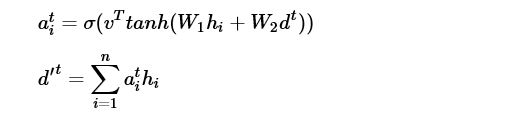
Where the Ws are learned matrices and v is a learned vector.    Then as the input to the t+1 state vector of the decoder we use the concatenation

atten4

The idea is this new state vector at time t+1 puts much more focus on the corresponding words in in the encoder string. This all happens in a function called seq2seq.attention_decoder that is called in another constructor function seq2seq.embedding_attention_seq2seq that wraps and an embedding around a graph generated by our MultiCellRNN graph builder to generate the final decoder graph.   These graphs are all stitched together in the Seq2SeqModel constructor.  It is fair to say that there are many levels of abstraction here that are used to build the decoder and link it to the encoder.  I am leaving out many details that are critical for the training such as the part that implements the bucket handler.   The final graph, in its most abstract form is pictured below in figure 3.

seq2seq_final

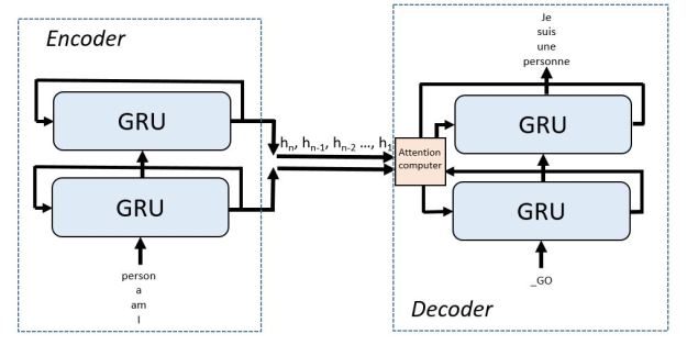
Figure 3.  The Translate.py sequence to sequence translator is based on a two level GRU cell encoder and an attention-augmented two level GRU cell decoder.  The input English is entered in reverse order as an optimization

Final Thoughts

As I have said above, I have not included all the details of how the seq2seq translator is put together, but I tried to include the highlights that I found most interesting.   I encourage you to dive into the code and discover the rest.   You will likely find some errors in what I described above.   If so, please let me know.

There is really a lot of exciting results that have come out in the last few years relating to RNNs.   For example, Lei Ba, Mnih and Kavukcuoglu demonstrated that RNNs with attention can be applied to interesting image analysis challenges, such as reading the house number from a street scene.   In “Teaching Machines to Read and Comprehend” Hermann et. al. excellent paper demonstrate the use of an attentive RNN build to answer simple questions about text.   I personally don’t think any RNN can pass a Turing test yet, so it ain’t A.I.  But these little statistical machines are certainly wonderful mimics and they can speak better French than I.

TensorFlow Meets Microsoft’s CNTK

Updated April 4, 1017.   Much of this material has been updated and improved and now appears as Chapter 10, Cloud Computing for Science and Engineering.  It can be accessed at the book’s website.

Update Nov 10, 2016.   Microsoft now has  a new release of CNTK.  We have a post now that provides a quick look at this new version.  Go read that one instead of this one.

Update Oct 25, 2016.    this post describes the early version of CNTK.  Microsoft just released a very nice new version called the cognitive toolkit.   I would not base your impression of CNTK  on the following post.   I’ll update this as soon as I have time.

———————–

CNTK is Microsoft’s Computational Network Toolkit for building deep neural networks and it is now available as open source on Github.   Because I recently wrote about TensorFlow I thought it would be interesting to study the similarities and differences between these two systems.   After all, CNTK seems to be the reigning champ of many of the image recognition challenges.   To be complete I should also look at Theano, Torch and Caffe.   These three are also extremely impressive frameworks.   While this study will focus on CNTK and TensorFlow I will try to return to the others in the future.   Kenneth Tran has a very nice top level (but admittedly subjective) analysis of all five deep learning tool kits here.  This will not be a tutorial about CNTK or Tensorflow.  Rather my goal is to give a high level feel for how they compare from the programmer’s perspective.  This is not a performance analysis, but rather a programming model analysis.  There is a lot of code here, so if you don’t like reading code, skip to the conclusions.

CNTK has a highly optimized runtime system for training and testing neural networks that are constructed as abstract computational graphs.   In that sense, CNTK is very much like TensorFlow.   However, there are some fundamental differences.   To illustrate these features and differences I will take two standard examples that are included with both systems and work through the approach taken by each system.   The first example is a not-too-deep convolutional neural net solution to the standard MNIST handwritten digit recognition example.  I will conclude with some comments about how they differ in their approach in the case of recurrent neural networks.

Both TensorFlow and CNTK are basically script-driven.   By this I mean that the construction of the neural network flow graph is described in a script and the training is done using some very clever automated processes.   In the case of TensorFlow the script is embedded in the Python language and Python operators can be used to control the flow of execution of the computational graph.   CNTK does not currently have a Python or C++ binding (though one is promised) so currently the control flow of the execution of the training and testing is highly choreographed.    As I will show, this is not as much of a limitation as it sounds.   There are actually two scripts associated with a CNTK network:  a configuration file that controls the training and test parameters and a network definition language file for constructing the network.

I’ll start with the description of the neural network flow graph because that is where the similarity to TensorFlow is the greatest.   There are two ways to define the network in CNTK.  One approach is to use the “Simple Network Builder” that will allow you to create some simple standard networks by specifying only a few parameter settings.    The other is to use their Network Definition Language (NDL).   The example here (taken directly from their download package in Github) uses NDL.    Below is a slightly abbreviated version of the Convolution.ndl file. (I have used commas to put multiple lines on one line to fit the page better.)

CNTK network graphs have a set of special nodes.  These are FeatureNodes and LabelNodes that describe the inputs and training labels,  CriterionNodes and EvalNodes that that are used for training and result evaluation, and OutputNodes that represent the outputs of the network.   I will describe these below as we encounter them.   At the top of the file we have a set of macros that are used to load the data (features) and labels.   As can be seen below we read images of the MNIST digits as features which are now arrays of floating point numbers that we have scaled by a small scalar constant.   The resulting array “featScaled” will be used as input to the network.

load = ndlMnistMacros

# the actual NDL that defines the network
run = DNN

ndlMnistMacros = [
    imageW = 28, imageH = 28
    labelDim = 10

    features = ImageInput(imageW, imageH, 1)
    featScale = Const(0.00390625)
    featScaled = Scale(featScale, features)
    labels = Input(labelDim)
]

DNN=[
    # conv1
    kW1 = 5, kH1 = 5
    cMap1 = 16
    hStride1 = 1, vStride1 = 1
    conv1_act = ConvReLULayer(featScaled,cMap1,25,kW1,kH1,hStride1,vStride1,10, 1)

    # pool1
    pool1W = 2, pool1H = 2
    pool1hStride = 2, pool1vStride = 2
    pool1 = MaxPooling(conv1_act, pool1W, pool1H, pool1hStride, pool1vStride)

    # conv2
    kW2 = 5, kH2 = 5
    cMap2 = 32
    hStride2 = 1, vStride2 = 1
    conv2_act = ConvReLULayer(pool1,cMap2,400,kW2, kH2, hStride2, vStride2,10, 1)

    # pool2
    pool2W = 2, pool2H = 2
    pool2hStride = 2,  pool2vStride = 2
    pool2 = MaxPooling(conv2_act, pool2W, pool2H, pool2hStride, pool2vStride)

    h1Dim = 128
    h1 = DNNSigmoidLayer(512, h1Dim, pool2, 1)
    ol = DNNLayer(h1Dim, labelDim, h1, 1)

    ce = CrossEntropyWithSoftmax(labels, ol)
    err = ErrorPrediction(labels, ol)

    # Special Nodes
    FeatureNodes = (features)
    LabelNodes = (labels)
    CriterionNodes = (ce)
    EvalNodes = (err)
    OutputNodes = (ol)
]

The network is defined in the block DNN.   The network consists of two convolutional-maxpooling layers followed by an all-to-all standard network with one hidden later of 128 nodes.

In convolutional layer one we have 5×5 convolutional kernels and we specify 16 of these (cMap1) for the parameter space.   The operator ConvReLULayer is actually a shorthand for another subnetwork defined in a macro file.

Algebraically we would like to represent the parameters of the convolution as a matrix W and a scale vector B so that if the input is X, the output of our network layer is of the form output = f(op(W, X) + B).   In this case the operator op is convolution and f is the standard relu function relu(x)=max(x,0).

The NDL code for the ConvReLULayer is given by

ConvReLULayer(inp, outMap, inWCount, kW, kH, hStride, vStride, wScale, bValue) = 
[
    convW = Parameter(outMap, inWCount, init="uniform", initValueScale=wScale)
    convB = Parameter(outMap, 1,        init="fixedValue", value=bValue)
    conv = Convolution(convW, inp, kW, kH, outMap, hStride,vStride,
                zeroPadding=false)
    convPlusB = Plus(conv, convB);
    act = RectifiedLinear(convPlusB);
]

The W matrix and B vector are defined as Parameters and they will be the entities that are given an initial value and then modified during training to define the final model.   In this case convW is a matrix with 16 rows of 25 columns B is a scale vector of length 16.   Convolution is a built-in function that has been set to not use zero padding.  This means that convolution over the 28×28 image will be centered on the 24 by 24 interior region and the result will be 16 variations of a 24×24 output sudo-image.

We next apply Maxpooling based on 2×2 regions and the result is now 12×12 by 16.

convo-nn-cntk

For the second convolutional layer we up the number of convolutional filters from 16 to 32.  This time we have 16 channels of input so the size of the W matrix is 32 rows  of 25×16 = 400 and the B vector for this layer is 32 long.   The convolution is now over the interior of the 12×12 frames so it is size 8×8 and we have 32 copies.    The second maxpooling step takes us to 32 frames of 4×4 or a result of size 32*16 = 512.

The final layers have the 512 maxpooling output and a hidden layer of 128 nodes to a final 10 node output defined by the two operators

DNNSigmoidLayer(inDim, outDim, x, parmScale) = [
    W = Parameter(outDim, inDim, init="uniform", initValueScale=parmScale)
    b = Parameter(outDim, 1,     init="uniform", initValueScale=parmScale)
    t = Times(W, x)
    z = Plus(t, b)
    y = Sigmoid(z)
]

DNNLayer(inDim, outDim, x, parmScale) = [
    W = Parameter(outDim, inDim, init="uniform", initValueScale=parmScale)
    b = Parameter(outDim, 1,     init="uniform", initValueScale=parmScale)
    t = Times(W, x)
    z = Plus(t, b)
]

As you can see these are defined by the standard linear algebra operators as W*x+b.

The final part of the graph definition is the cross entropy and error nodes followed by a binding of these to the special node names.

We will define the training process soon, but first it is fun to compare this to the construction of a very similar network in TensorFlow.   We described this in a previous post but here it is again.   Notice that we have the same set of variables as we did with CNTK except they are called variables here and parameters in CNTK.   The  dimensions are also slightly different.  The convolutional filters 5×5 in both cases but we have 16 copies in the first stage and 32 in the second in CNTK and 32 in stage one and 64 in stage two in the TensorFlow example.

def weight_variable(shape, names):
  initial = tf.truncated_normal(shape, stddev=0.1)
  return tf.Variable(initial, name=names)

def bias_variable(shape, names):
  initial = tf.constant(0.1, shape=shape)
  return tf.Variable(initial, name=names)

x = tf.placeholder(tf.float32, [None, 784], name="x")

sess = tf.InteractiveSession()

W_conv1 = weight_variable([5, 5, 1, 32], "wconv")
b_conv1 = bias_variable([32], "bconv")
W_conv2 = weight_variable([5, 5, 32, 64], "wconv2")
b_conv2 = bias_variable([64], "bconv2")
W_fc1 = weight_variable([7 * 7 * 64, 1024], "wfc1")
b_fc1 = bias_variable([1024], "bfcl")
W_fc2 = weight_variable([1024, 10], "wfc2")
b_fc2 = bias_variable([10], "bfc2")

The network construction is also almost identical.

def conv2d(x, W):
  return tf.nn.conv2d(x, W, strides=[1, 1, 1, 1], padding='SAME')

def max_pool_2x2(x):
  return tf.nn.max_pool(x, ksize=[1, 2, 2, 1],
                        strides=[1, 2, 2, 1], padding='SAME')

#first convolutional layer
x_image = tf.reshape(x, [-1,28,28,1])
h_conv1 = tf.nn.relu(conv2d(x_image, W_conv1) + b_conv1)
h_pool1 = max_pool_2x2(h_conv1)
#second convolutional layer
h_conv2 = tf.nn.relu(conv2d(h_pool1, W_conv2) + b_conv2)
h_pool2 = max_pool_2x2(h_conv2)
#final layer
h_pool2_flat = tf.reshape(h_pool2, [-1, 7*7*64])
h_fc1 = tf.nn.relu(tf.matmul(h_pool2_flat, W_fc1) + b_fc1)
h_fc1_drop = tf.nn.dropout(h_fc1, keep_prob)
y_conv=tf.nn.softmax(tf.matmul(h_fc1_drop, W_fc2) + b_fc2)

The only differences are that the convolutional operators here are defined with padding so the output of the first convolutional operator had dimensions of 28 by 28 flowed by a pooling reduction to 14 by 14.  The second convolutional operator and max pooling reduces this to 7×7, so the input to the final layer is 7x7x64 = 3136 with 1024 hidden nodes (with a relu instead of a sigmoid function).   (For training purposes the last stage uses a probabilistic dropout function that randomly set values to zero.   If keep_prob = 1, this is a no-op. )

convolutional

Network Training

The way network training is specified in CNTK differs substantially from the TensorFlow approach.  The training and testing is specified in a file called convolution.config.  Both CNTK and TensorFlow use a symbolic analysis of the flow graph to compute the gradient of the network for use in gradient decent training algorithms.  The CNTK team has a very nice “book” that describes a great deal about how the gradients are computed.   Currently CNTK only supports one learning method: Mini-batch Stochastic Gradient Decent, but they promise to add more in the future.  He, Zhang, Ren and Sun have a lovely paper that describes how they train extremely deep (up to 1000 layers) networks using a nested residual reduction method reminiscent of algebraic multi-grid, so it will be interesting to see if that method makes its way into CNTK.  An abbreviated version of the config file is shown below.

command = train:test
modelPath = "$ModelDir$/02_Convolution"
ndlMacros = "$ConfigDir$/Macros.ndl"

train = [
    action = "train"
    NDLNetworkBuilder = [
        networkDescription = "$ConfigDir$/02_Convolution.ndl"
    ]

    SGD = [
        epochSize = 60000
        minibatchSize = 32
        learningRatesPerMB = 0.5
        momentumPerMB = 0*10:0.7
        maxEpochs = 15
    ]

    reader = [
        readerType = "UCIFastReader"
        file = "$DataDir$/Train-28x28.txt"

        features = [
            dim = 784
            start = 1
        ]

        labels = [
		    # details deleted
        ]
    ]
]
test = [
   ….
]

The command line indicates the sequence to follow:  train then test.   Various file paths are resolved and then the train block specifies the network to be trained and the parameters for the Stochastic Gradient Decent (SGD).  A reader block specifies the way the “features” and “labels” from the network NDL file are read.   A test block is also included to define the parameters of the test.

Running this on a 16-core (non-GPU) linux VM took 62.95 real-time minutes to do the train and test and 999.01 minutes of user time and 4 minutes of system time.    The user time indicated that all 16 cores were all very busy (999/63 = 15.85).   Of course this means little as CNTK is designed for parallelism and massive GPU support is the true design point idea.

The training used by TensorFlow is specified much more explicitly in the Python control flow.   However, the algorithm is also a gradient based method called Adam introduced by Kingma and Ba.    Tensorflow has a number of gradient based optimizers in the library, but I did not try any of the others.

As can be seen below, the cross_entropy is defined in the standard way and fed to the optimizer to produce a “train_step” object.

y_ = tf.placeholder(tf.float32, [None, 10])
cross_entropy = -tf.reduce_sum(y_*tf.log(y_conv))
train_step = tf.train.AdamOptimizer(1e-4).minimize(cross_entropy)
correct_prediction = tf.equal(tf.argmax(y_conv,1), tf.argmax(y_,1))
accuracy = tf.reduce_mean(tf.cast(correct_prediction, "float"))
sess.run(tf.initialize_all_variables())
for i in range(20000):
  batch = mnist.train.next_batch(50)
  train_step.run(feed_dict={x: batch[0], y_: batch[1], keep_prob: 0.5})

print("test accuracy %g"%accuracy.eval(feed_dict={
    x: mnist.test.images, y_: mnist.test.labels, keep_prob: 1.0}))

Then for 20000 iterations the python program grabs a batch of 50 and runs the train_step with 50% random dropout.  The test step is to evaluate the accuracy subgraph on the entire test set.

Aside from the magic of the automatic differentiation and the construction of the Adam optimizer trainer, this is all very straightforward.   I also ran this on the same 16 core server with the same data as was used for the CNTK case.   Much to my surprise the real time was almost exactly the same as CNTK.   The real time was 62.02 minutes, user time 160.45 min, so much less parallelism was exploited.    I don’t believe these numbers mean much.   Both CNTK and Tensor flow are designed for large scale GPU execution and they are not running exactly the same training algorithm.

Recurrent Neural Nets with CNTK and TensorFlow

Recurrent Neural Networks (RNNs) are widely used in language modeling such as predicting the next word you are going to type when texting or in automatics translation systems.   (see Andrej Karpathy’s blog for some great examples.) It is really a lovely idea. The input to the system is a word (or set of words) along with the state of the system based on words seen so far and the output is a predicted word list and a new state of the system as shown in Figure 1.

rnn_basic

Figure 1.

There are, of course, many variations of the basic RNN.   One of the most popular is the Long-Short Term Memory (LSTM) version that is defined by the equations

lstm_eqn

Figure 2. LSTM Equations (taken from the CNTK book)

where sigma   is the sigmoid function.

If you want to read a great blog article about LSTMs and how they work, I recommend this one by Christopher Olah.   In fact, he has a diagram that makes it a bit easier to see the flow of the equations above.  I had to modify it a tiny bit to fit the CNTK version of the equations and the result is shown in Figure 3.

lstm_fig

Figure 3.  Adapted from Christopher Olah’s excellent article.

The notation in the picture uses sigmoid and tanh boxes and concatenated variables to represent this expression.

sigmoid

As can be seen, this is the form of the equations in figure 2 where the Ws and the bs are the learned weights.

CNTK version

Below is the network definition language specification for the LSTM graph.   There are two things to notice here.    The first is the way the recurrence is handled directly in the network using a delay operator called “PastValue” that takes variable, its dimension and a time delay value and returns a buffered copy of that value.   The second thing to see is the way the W matrix is handled and how it differs from our concatenated operator describe above and in Figure 3.   Here they “stack” all the Ws that belong to x and all the Ws that belong to h and a stack of b values.   They then compute one W*x and one W*h and add them and then add b.   They then use a row slice operator to pull them apart to be used in the separate sigmoid functions.   Also note that they use the fact the Ws for c are all diagonal matrices.

LSTMPComponent(inputDim, outputDim, cellDim, inputx, cellDimX2, cellDimX3, cellDimX4) = [
        wx = Parameter(cellDimX4, inputDim,  init="uniform", initValueScale=1);
        b = Parameter(cellDimX4,  1,         init="fixedValue", value=0.0);
        Wh = Parameter(cellDimX4, outputDim, init="uniform", initValueScale=1);

        Wci = Parameter(cellDim, init="uniform", initValueScale=1);
        Wcf = Parameter(cellDim, init="uniform", initValueScale=1);
        Wco = Parameter(cellDim, init="uniform", initValueScale=1);

        dh = PastValue(outputDim, output, timeStep=1);
        dc = PastValue(cellDim, ct, timeStep=1);

        wxx = Times(wx, inputx);
        wxxpb = Plus(wxx, b);
        
        whh = Times(wh, dh);

        wxxpbpwhh = Plus(wxxpb,whh)
        
        G1 = RowSlice(0, cellDim, wxxpbpwhh)
        G2 = RowSlice(cellDim, cellDim, wxxpbpwhh)
        G3 = RowSlice(cellDimX2, cellDim, wxxpbpwhh);
        G4 = RowSlice(cellDimX3, cellDim, wxxpbpwhh);

        Wcidc = DiagTimes(Wci, dc);
        it = Sigmoid (Plus ( G1, Wcidc));

        bit = ElementTimes(it, Tanh( G2 ));

        Wcfdc = DiagTimes(Wcf, dc);
        ft = Sigmoid( Plus (G3, Wcfdc));

        bft = ElementTimes(ft, dc);

        ct = Plus(bft, bit);

        Wcoct = DiagTimes(Wco, ct);
        ot = Sigmoid( Plus( G4, Wcoct));

        mt = ElementTimes(ot, Tanh(ct));

        Wmr = Parameter(outputDim, cellDim, init="uniform", initValueScale=1);
        output = Times(Wmr, mt); 
    ]

The TensorFlow version

The TensorFlow version of the LSTM recurrent neural network is very different from the CNTK version.   While they both execute the same underling set of equations the way it is represented in TensorFlow make strong use of the Python control flow.    The conceptual model is simple.  We create a LSTM cell and define a “state” which is input to the cell and also an output.   In pseudo code:

cell = rnn_cell.BasicLSTMCell(lstm_size)
# Initial state of the LSTM memory.
state = tf.zeros([batch_size, lstm.state_size])

for current_batch_of_words in words_in_dataset:
    # The value of state is updated after processing each batch of words.
    output, state = cell(current_batch_of_words, state)

This is a nice pseudo code version of figure 1 taken from the tutorial.   The devil is in the very subtle details.   Remember that most of the time python code in Tensor flow is about building the flow graph, so we have to work a bit harder to build the graph with the cycle that we need to train and execute.

It turns out that the greatest challenge is defining how we can create and reuse the weight matrices and bias vectors inside a graph with a cycle.   CNTK uses the operator “PastValue” to create the needed cycle in the graph.  TensorFlow uses the literal recurrence above and a very clever variable save and recall mechanism to accomplish the same thing.   The moral equivalent of “PastValue” in Tensorflow is a function called tf.get_variable( “name”, size, initializer = None) whose behavior depends  upon a flag called “reuse” associated with the current variable scope.  If reuse==False and no variable already exists by that name in this scope then get_variable returns a new variable with that name and uses the initializer to initialize it.  Otherwise it returns an error.  If reuse == True then get_variable returns the previously existing variable by that name.  If no such variable exists, it returns an error.

To illustrate how this is used below is a simplified version of one of the functions in TensorFlow used to create the sigmoid function from eq. 1 above.  It is just a version of W*x+b where x is a list [a, b, c, …].

def linear(args, output_size, scope=None):
   #Linear map: sum_i(args[i] * W[i]), where W[i] is a variable.
   with vs.variable_scope(scope):
    matrix = vs.get_variable("Matrix", [total_arg_size, output_size])
    res = math_ops.matmul(array_ops.concat(1, args), matrix)
    bias_term = vs.get_variable(
        "Bias", [output_size],
        initializer=init_ops.constant_initializer(1.))
  return res + bias_term

Now to define the BasicLSTMCell we can write it roughly as follows.   (To see the complete versions of these functions look at rnn_cell.py in the TensorFlow Github repository.)

class BasicLSTMCell(RNNCell):
  def __call__(self, inputs, state, scope=None):
    with vs.variable_scope(scope): 
      c, h = array_ops.split(1, 2, state)
      concat = linear([inputs, h], 4 * self._num_units)
      i, j, f, o = array_ops.split(1, 4, concat)
      new_c = c * sigmoid(f) + sigmoid(i) * tanh(j)
      new_h = tanh(new_c) * sigmoid(o)
   return new_h, array_ops.concat(1, [new_c, new_h])

As you can see, this is a fairly accurate rendition of the diagram in Figure 3.  You will notice the operator split above is the counterpart to the rowslice operation in the CNTK version.

We can now create instances of a recurrent neural network that can be used for training and using the same variable scope we can create another one to use for testing that share the same W and b variables.  The way this is done is shown in ptb_word_lm.py in the TensorFlow tutorials for recurrent neural nets.  There are two additional points worth observing.  (I should say they were critical for me to understand this example.)   They create a class lstmModel that can be used to build the networks for training and test.

class lstmModel:
  def __init__(self, is_training, num_steps):
    self._input_data = tf.placeholder(tf.int32, [batch_size, num_steps])
    self._targets = tf.placeholder(tf.int32, [batch_size, num_steps])
 	cell = rnn_cell.BasicLSTMCell(size, forget_bias=0.0)
    outputs = []
    states = []
    state = self._initial_state
    with tf.variable_scope("RNN"):
      for time_step in range(num_steps):
        if time_step > 0: 
            tf.get_variable_scope().reuse_variables()
        (cell_output, state) = cell(inputs[:, time_step, :], state)
        outputs.append(cell_output)
        states.append(state)
        … many details omitted …

Where this is used is in the main program were we create a training instance and a test instance (actually there is a third instance which I am skipping to keep this as simple as possible).

with tf.variable_scope("model", reuse=None, initializer=initializer):
  m = PTBModel(is_training=True, 20)
with tf.variable_scope("model", reuse=True, initializer=initializer):
   mtest = PTBModel(is_training=False, 1)

What is happening here is that the instance m is created with 20  steps with no reuse initially.  As you can see from the initializer above that will cause the loop to unroll 20 copies of the cell in the graph and after the first iteration the reuse flag is set to True, so all instances will share the same W and b.   The training works on this unrolled version.   The second version mtest has reuse = True and it only has one instance of the cell in the graph.   But  the variable scope is the same as m, so it shares the same trained variables as m.

Once trained, we can invoke the network with a kernel like the following.

cost, state = sess.run([mtest.cost, mtest.final_state],
                                 {mtest.input_data: x,
                                  mtest.targets: y,
                                  mtest.initial_state: state})

Where x and y are the inputs. This is far from the complete picture of the tutorial example. For example, I have not gone into the training at all and the full example uses a stacked LSTM cell and a dropout wrapper. My hope is that the detail I have focused on here will help the reader understand the basic structure of the code.

Final Observations

I promised a programming model comparison of the two systems.    Here are some top level thoughts.

  1. TensorFlow and CNTK are very similar for the simple convolutional neural network example.  However, I found the TensorFlow version easier to experiment with because it is driven by python. I was able to load it as a IPython notebook and try different things.  With CNTK one needed to completely understand how to express things with the configuration file.   I found that difficult.   With TensorFlow I was able to write a simple k-means clustering algorithm (see my previous post on Tensorflow).   I was unable to do this with CNTK and that may be due to my cluelessness rather than a limit of CNTK.  (If somebody knows how to do it, I would appreciate a tip.)
  2. In the case of the LSTM recurrent neural network, I found the CNTK version to be completely transparent.   In the case of Tensorflow I found the top level idea very elegant, but I also found it very difficult to understand all the details because of the clever use of the variable scoping and variable sharing.   I had to dig very deep to understand how it worked.   And it is not clear that I have it all yet!   I did find one trivial bug in the Tensorflow version that was easy to fix and I am not convinced that the variable scoping and reuse flags, which are there to solve an encapsulation problem, are the best solutions.  But the good think about TensorFlow is that I can easily experiment with alternatives.
  3. I must also say that the CNTK book and the TensorFlow tutorials are both excellent introductions to the high level concepts.  I am sure more detailed, deep-dive books will come out soon.

I am also convinced that as both systems mature they will improve and become easier to program.   I did not discuss performance, but CNTK is the current champ in terms of speed on some difficult challenges.  But with the rapid evolution of these systems I expect to see the competition to heat up.