In a previous post I talked about using Mesosphere on Azure for scaling up many-tasks parallel jobs and I promised to return to Kubernetes when I figured out how to bring it up.   Google just made it all very simple with their new Google Cloud container services.   And, thanks to their good tutorials, I learned about a very elegant way to do remote procedure calls using another open source tool called Celery.

So let me set the stage with a variation on an example I have used in the past.   Suppose we have 10000 scientific documents that are stored in the cloud.   I would like to use a simple machine learning method to classify each of these by topic.    I would like to do this quickly as possible and, because the analysis of each document is independent of the others, I can try to process as many as possible in parallel.  This is the basic “many task” parallel model and one of the most common uses of the cloud for scientific computing purposes.      To do this we will use the Celery distributed task queue mechanism to take a list of our documents and send each one to a work queue where the tasks will be parceled out to workers who will do the analysis and respond.

The Google Cloud Container Service and a few words about Kubernetes.

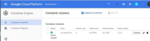
Before getting into the use of Celery and the analysis program, let’s describe the Google Cloud Container Service and a bit about Kubernetes.   Getting started is incredibly easy.   Google has a small free trial account which is sufficient to do the experiments described.  Go to http://cloud.google.com and sign in or create an account.  This will take you to the “console” portal. The first thing you need to do is to create a project. In doing so it will be assigned an id which is a string of the form “silicon-works-136723”.    There is a drop down menu on the left end of the blue banner at the top of the page.  (Look for three horizontal bars.) This allows you to select the type of service you want to work on.     Select the “Container Engine”.  On the “container clusters” page there is a link that will allow you to create a cluster.   With the free account you cannot make a very big cluster.   You are limited to about 4 dual core servers.   If you fill in the form and submit it, you will soon have a new cluster.  There is a special icon of the form “>_” in the blue banner.  Clicking on that icon will create an instance of a “Cloud Shell” that will be automatically authenticated to your account.   The page you will see should resemble Figure 1 below.   The next thing you need to do is to authenticate your cloud shell with your new cluster.   By selecting your container and clicking on the “connect” button to the right you will get the code to paste into the cloud shell.  The result should now look exactly like Figure 1.

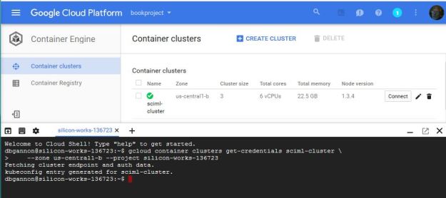
Figure 1.   Creating a Google cloud cluster and connecting the cloud shell to it.

Interacting with Kubernetes, which is now running on our small cluster, is through command lines which can be entered into the cloud shell.   Kubernetes has a different, and somewhat more interesting architectures than other container management tools.   The basic unit of scheduling in Kubernetes is  launching pods. A pod consists of a set of one or more Docker-style containers together with a set of resources that are shared by the containers in that pod.  When launched a pod resides on a single server or VM.   This has several advantages for the containers in that pod.   For example, because the containers in a pod are all running  on the same VM, the all share the same IP and port space so the containers can find each other through conventional means like “localhost”.   They can also share storage volumes that are local to the pod.

To start let’s consider a simple single container pod to run the Jupiter notebook.  There is a standard Docker container that contains Jupyter and the scipy software stack.  Using the Kubernetes control command kubectl we can launch Jupyter and expose its port 8888 with the following statement.

$ kubectl run jupyter --image=jupyter/scipy-notebook --port=8888

To see that it is up and running we can issue the command “kubectl get pods” which will return the status of all of our running pods.   Though we have launched jupyter it is still not truly visible.   To do that we will associate a load balancer with the pod.   This will expose the port 888 to the open Internet.

$ kubectl expose deployment jupyter --type=LoadBalancer

Once that has been run you can get the IP address for jupyter from the “LoadBalancer Ingress:” field of the service description when you run the following.   If it doesn’t appear, try again.

$ kubectl describe services jupyter

One you have verified that it is working at that address on port 8888, you should shut it down immediately because, as you can see, there is no security with this deployment.  Deleting a deployment is easy.

$ kubectl delete deployment jupyter

 There is another point that one must be aware of when building containers that need to directly interact with the google cloud APIs.  To make this work you will need to get application default credentials to run in your container.   For example if you container is going to interact with the storage services you will need this.   To get the default application credentials follow the instructions here.  We will say a few more words about this below.

The Analysis Example in detail.

Now to describe  Celery and how to use Celery and Kubernetes in the many-task scenario described above.

To use Celery we start with our analysis program.   We have previously described the analysis algorithms in detail in another post, so we won’t duplicate that here.  Let’s start by assuming we have a function predict(doc) that takes a document as a string as an argument and returns a string containing the result from our trained machine learnging classifiers.  Our categories are “Physics”, “Math”, “Bio”, “Computer Science” and “Finance” and the result from each classifier is simply the category that that classifier determines to be the most likely correct answer.

Celery is a distributed remote procedure call system for Python programs.   The Celery view of the world is you have a set of worker processes running on remote machines and a client process that is invoking functions that are executed on the remote machines.   The workers and the clients all coordinate through a message broker running somewhere else on the network.

Here we use a RabbitMQ service that is running on a Linux VM on the NSF JetStream cloud as illustrated in Figure 2.

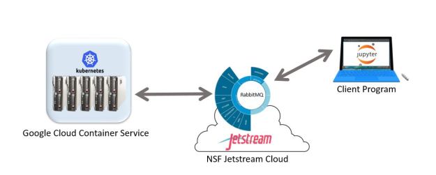
Figure 2.  Experimental Configuration with Celery workers running on Kubernetes in the Google Cloud Container Service,  the RabbitMQ broker running in a VM on the NSF Jetstream Cloud and a client program running as a notebook on a laptop.

The code block below illustrates the basic Celery worker template.    Celery is initialized with a constructor that takes the name of the project and a link to the broker service which can be something like a Redis cache or MongoDB.   The main Celery magic is invoked with a special Python “decorator” associated with the Celery object as shown in the predictor.py file below.

from celery import Celery
app = Celery('predictor', backend='amqp')

#Now initialize and load all the data structure that will be constant 
#and recused for each analysis.  In our case this will include
#all the machine learning models that were trained on the data 
#previously. And create a main worker function to invoke the models.  
def invokeMLModels(statement):
    ....
	return analysis
	
#define the functions we will call remotely here
@app.task
def predict(statement):
	prediction = invokeMLModels(statement)
	return [prediction]

What this decorator accomplishes is to wrap the function in a manner that it can be invoked by a remote client.   To make this work we need create a Celery worker from our predictor.py file with the command below which registers a worker instance as a listener on the RabbitMQ queue.

>celery worker -A predictor -b 'amqp://guest@brokerIPaddr'

Creating a client program for our worker is very simple.   It is similar to the worker template except that our version of the predict( ) function does nothing because we are going to invoke it with the special Celery apply_async( ) method that will push the argument to the broker queue and return control immediately to the client.   The object that is returned from this call is similar to what is sometimes called a “future” or a “promise” in the programming language literature.  What it is a placeholder for the returned value.   Once we attempt to evaluate the get() method on this object our client will wait until a reply is returned from the remote worker that picked up the task.

from celery import Celery
app = Celery('predictor', broker='amqp://guest@brokerIPaddr', backend='amqp')

@app.task
def predict(statement):
	return ["stub call"]
	
res = predict.apply_async(["this is a science document ..."])

print res.get()

Now if we have 10000 documents to analyze we can send them in sequence to the queue as follows.

#load all the science abstracts into a list
documents = load_all_science_abstracts()

res = []
for doc in documents:
   res.append(predict.apply_async([doc])

#now wait for them all to be done
predictions = [result.get() for result in res]
#now do an analysis of the predictions

Here we push each analysis task into the queue and save the async returned objects in a list.  Then we create a new list by waiting for each prediction value to be returned.   Our client can run anywhere there is Internet access.  For example this one was debugged on a Jupyter instances running on a laptop.  All you need to do is “pip install celery” and run Juypter.

There is much more to say about Celery and the interested reader should look at the Celery Project site for the definitive guide. Let us now turn to using this with Kubernetes.  We must first create a container to hold the analysis code and all the model data.   For that we will need a Docker file and a shell script to correctly launch celery one the container is deployed.   For those actually interested in trying this, all the files and data are in OneDrive here.   The Docker file shown below has more than we need for this experiment.

# Version 0.1.0
FROM ipython/scipystack
MAINTAINER yourdockername "youremail"
RUN easy_install celery
RUN pip install -U Sphinx
RUN pip install Gcloud
RUN easy_install pattern
RUN easy_install nltk
RUN easy_install gensim
COPY bookproject-key.json /
COPY models /
COPY config /
COPY sciml_data_arxiv.p /
COPY predictor.py /
COPY script.sh /
ENTRYPOINT ["bash", "/script.sh"]

To build the image we first put all the machine learning configuration files in a directory called config and all the learned model files in a directory called models.  At same level we have the predictor.py source.   For reasons we will explain later we will also include the full test data set: sciml_data_arxiv.p. The Docker build starts with the ipython/scipystack container.   We then use easy_install to install Celery as well as four packages used by the ML analyzers: pattern, nltk and gensim.   Though we are not going to use the Gcloud APIs here, we include them with a pip install.   But to make that work we need an updated copy of Sphinx.  To make the APIs work we would need our default client authentication keys.   They are stored in a json file called bookproject-key.json that was obtained from the Gcloud portal as described previously.   Finally we copy all of the files and directory to the root path ‘/’.  Note that the copy from a directory is a copy of the all contained files to the path ‘/’ and not to a new directory.   The ENTRYPOINT runs our script which is shown below.

cp /predictor.py .
export C_FORCE_ROOT='true'
export GOOGLE_APPLICATION_CREDENTIALS='/bookproject-key.json'
echo $C_FORCE_ROOT
celery worker -A predictor -b $1

Bash will run our script in a temp directory, so we need to copy our predictor.py file to that directory.  Because our bash is running as root, we need to convince Celery that it is o.k. to do that.  Hence we export C_FORCE_ROOT as true.  Next, if we were using the Gcloud APIs we need to export the application credentials.   Finally we invoke celery but this time we use the -b flag to indicate that we are going to provide the IP address of the RabbitMQ amqp broker as a parameter and we remove it from the explicit reference in the predictor.py file.  When run the predictor file will look for all the model and configuration data in ‘/’.   We can now build the docker image with the command

>docker build -t “yourdockername/predictor” .

And we can test the container on our laptop with

>docker run -i -t “yourdockername/predictor ‘amqp://guest@rabbitserverIP’

Using “-i -t” allows you to see any error output from the container.   Once it seems to be working we can now push the image to the docker hub.   (to use our version directly, just pull dbgannon/predictor)

We can now return to our Google cloud shell and pull a version of the container there.   If we want to launch the predictor container on the cluster, we can do it one at a time with the “kubectl run” command.  However Kubernetes has a better way to do this using a pod configuration file where we can specify the number of pod instances we want to create.  In the file below, which we will call predict-job.json we specify a job name, the container image in the docker hub,   and the  parameter to pass to the container to pass to the shell script.   We also specify the number of pods to create.   In this case that is 6 as identified in the “parallelism” parameter.

apiVersion: batch/v1
kind: Job
metadata:
   name:predict-job
spec:
   parallelism: 6
   template:
        metadata:
            name: job-wq
       spec:
            containers:
                  - name: c
                  image: dbgannon/predictor
                  args: ["amqp://guest@ipaddress_of_rabbitmq_server"]
          restartPolicy: OnFailure

One command in the cloud shell will now launch six pods each running our predictor container.

$kubectl create -f predict-job.json 

Some Basic Performance Observations.

When using many tasks system based on a distributed worker model there are always three primary questions about the performance of the system.

1. What is the impact of wide-area distribution on the performance?
2. How does performance scale with the number of worker containers that are deployed? More specifically, if we N workers, how does the system speed up as N increases?    Is there a point of diminishing return?
3. Is there a significant per/task overhead that the system imposes?  In other words, If the total workload is T and if it is possible to divide that workload into k tasks each  of size T/k , then what is the best value of k that will maximize performance?

Measuring the behavior of a Celery application as a function of the number workers is complicated by a number of factors.   The first concern we had was the impact of widely distributing the computing resources on the overall performance.   Our message broker (RabbitMQ) was running in a virtual machine in Indiana on the JetStream cloud.   Our client was running a Jupyter notebook on a laptop and the workers were primarily on the Midwest Google datacenter and on a few on other machines in the lab.   We compared this to a deployment where all the workers, the message broker and the client notebook were all running together on the Google datacenter.   Much to our surprise there was little difference in performance between the two deployments.   There are two ways to view this result.   One way is to say that the overhead of wide area distribution was not significant.   The other way to say this is that the overhead of wide area distribution was negligible compared to other performance problems.

A second factor that has an impact on performance as a function of the number of workers is the fact that a single Celery worker may have multiple threads that are responding to asynchronous function calls.   While we monitored the execution we noticed that the number of active threads in one worker could change over time. This made performance somewhat erratic.  Celery’s policy is that it will never have more threads than the number of available cores, so to limit the thread variability we ran workers in container pods on VMs with only one core.

Concerning the question of the granularity of the work partitioning we configured the program so that a number of documents could be processed in one invocation and this number could be set remotely.    By taking a set of 1000 documents and a fixed set of workers, we divided the document set into blocks of size K where K ranged from 1 to 100.   In general, larger blocks were better because the number of Celery invocations was smaller, but the difference was not great.   Another factor involved Celery’s scheduling for deciding which worker get the next invocation.   For large blocks this was not the most efficient because this left holes in the execution schedule when workers were occasionally idle while another was over scheduled.   For very small blocks these holes tended to be small.   We found that a value of K=2 gave reasonably consistent performance.

Finally to test scalability we used three different programs.

1. The document topic predictor described above where each invocation classified two documents.
2. A simple worker program that does no computation but just sleeps for 10 seconds before returning a “hello world” string.
3. A worker that computes part of the Euler sequence sum(1/i**2, i=1..n) where n = 10⁹ .   Each worker computes a block of 10⁷ terms of the sequence and the 100 partial results are added together to get the final result  (which approximates pi²/6  to about 7 decimal places).

The document predictor is very computational intensive and uses some rather large data matrices for the trained machine learning models.   The size of these arrays are about 150 megabytes total.  While this does fit in memory, the computation is going to involve a great deal of processor cache flushing and there may be memory paging effects.   The example that computes the Euler sum requires no data other than the starting point index and the size of the block to sum.   It is pure computation and it will have no cache flushing or memory paging effects, but it will keep the CPU very busy.   The “sleep” example leaves the memory and the CPU completely idle.

We ran all three with one to seven workers.   (6 workers using 6 cores from the small Google demo account and one on another other remote machine).    To compare the results, we computed the time for each program on one worker and plotted the speed-up ratio for 2, 3, 4, 5, 6 and 7 workers.   The results are shown in the graphs below.

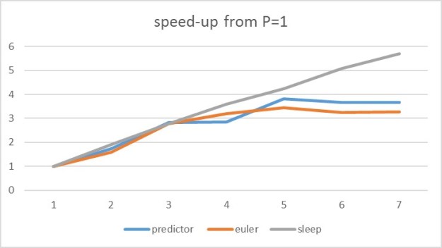
Figure 3.  Performance as speed-up for each of the three applications with up to 7 workers.

As can be seen, the sleeper scales linearly in the number of workers.   In fact, when executed on multi-core machines it is almost super-linear because of the extra threads that can be used.  (It is very easy for a large number of threads to sleep in parallel.)   On the other hand, the predictor and the Euler examples reached a maximum speed up with around five workers.  Adding more worker pods to the servers did not show improvement because these applications are already very compute intensive.    This was a surprise as we expect all three experiments to scale well beyond seven workers.  Adding more worker pods to the servers did not show improvement because these applications are already very compute intensive.   When looking for the cause of this limited performance, we considered the possibility that the RabbitMQ broker was a bottleneck, but our previous experience with it has allowed us to scale applications to dozens of concurrent reader and writers.   We are also convinced that the Google Container Engine performed extremely well and it was not the source of any of these performance limitations. We suspect (but could not prove) that the Celery work distribution and result gathering mechanisms have overheads that limit scalability as the number of available workers grows.

Conclusion

Google has made it very easy to deploy containerized applications using Kubernetes on their cloud container service.  Kubernetes has some excellent architectural features that allow multiple containers to be co-located on a single server within a pod.   We did not have time here to demonstrate this, but their documentation gives some excellent examples.

Celery is an extremely elegant way to do remote procedure calls in Python.  One only needs to define the function and annotate it with a Celery object.   It can then be remotely invoked with an asynchronous call that returns control to the caller.  A future like object is returned.  By calling a special method on the returned object the caller will pause until the remote call completes and the value is provided to the caller.

Our experiments demonstrated that Celery has limited scalability if it is used without modification and with the RabbitMQ message broker.   However, celery has many parameters and it may be possible that the right combinations will improve our results.  We will report any improved results we discover in a later version of this document.