Tag Archives: Azure

Streaming Events to AzureML Through Azure Stream Analytics


UPDATE!  Microsoft has just recently released a much better way to integrate Azure Machine Learning with Azure Stream Analytics.  You can now call an AzureML service directly from the SQL query in the stream analytics system.  This means you don’t need the message bus and microservice layer I describe below.   Check out the blog by Sudhesh Suresh and the excellent tutorial from Jeff Stokes.   I will do a performance analysis to compare this method to the one below, but I will wait until the new feature comes out of “preview” mode :).   I will also use a better method to push events to the eventhub.


Doing sophisticated data analytics on streaming data has become a really interesting and hot topic.   There is a huge explosion of research around this topic and there are a lot of new software tools to support it.  Amazon has its new Kinesis system,  Google has moved from MapReduce to Cloud DataFlow, IBM has Streaming Analytics on their Bluemix platform and Microsoft has released Azure Stream Analytics.  Dozens of other companies that use data streaming analytics to make their business work have contributed to the growing collection of open source of tools.   For example LinkedIn has contributed the original version of Apache Kafka and Apache Samza and Yahoo contributed Storm.  And there are some amazing start-ups that are building and supporting important stream analytics tools such as Flink from Data-Artisans. Related university research includes systems like Neptune from Colorado State.  I will post more about all of these tools later, but in this article I will describe my experience with the Microsoft EventHub, Stream Analytics and AzureML.   What I will show below is the following

  1. It is relatively easy to build a streaming analytics pipeline with these tools.
  2. It works, but the  performance behavior of the system is a bit uneven with long initial latencies and a serious bottleneck which is probably the result of small size of my experiment.
  3. AzureML services scale nicely
  4. Finally there are some interesting ways in which blocking can greatly improve performance.

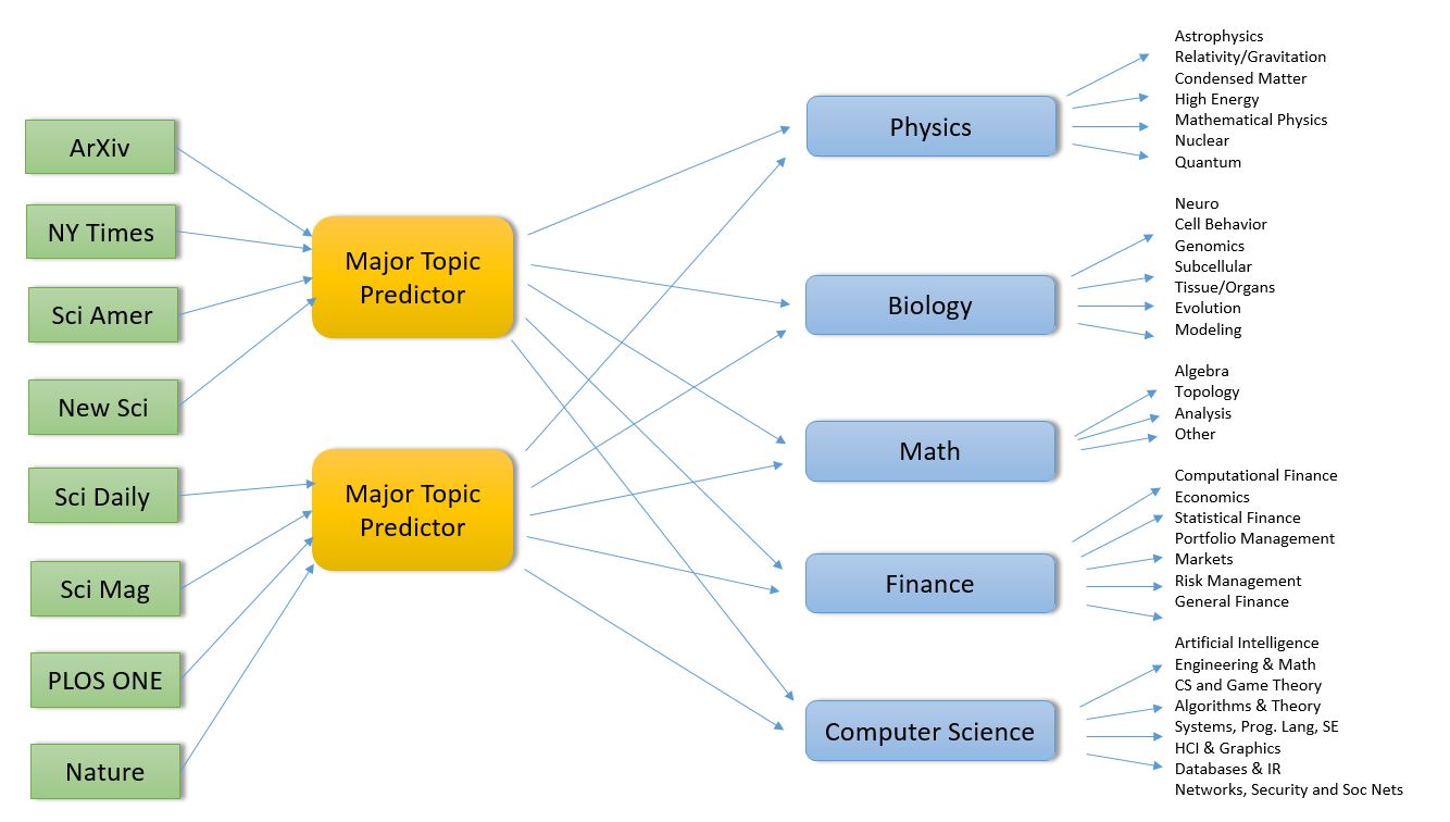
In a previous post I described how to use AzureML to create a version of a science document analyzer that I originally put together using Python Scikit-Learn, Docker and Mesosphere.  That little project is described in another post.   The streaming challenge here is very simple.   We have data that comes from RSS feeds concerning the publication of scientific papers.  The machine learning part of this is to use the abstract of the paper to automatically classify the paper into scientific categories.  At the top level these categories are “Physics”, “math”, “compsci”, “biology”, “finance”.    Big streaming data challenges that you find in industry and science involve the analysis of events that may be large and arrive at the rate of millions per second.   While there are a lot of scientists writing lots papers, they don’t write papers that fast.   The science RSS feeds I pull from are generating about 100 articles per day.  That is a mere trickle.  So to really push throughput experiments I grabbed several thousands of these records and wrote a simple server that would push them as fast as possible to the analysis service.

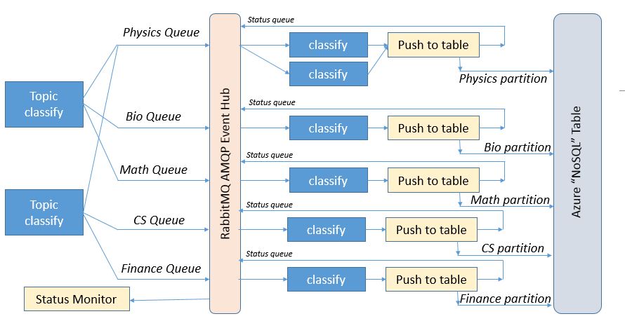
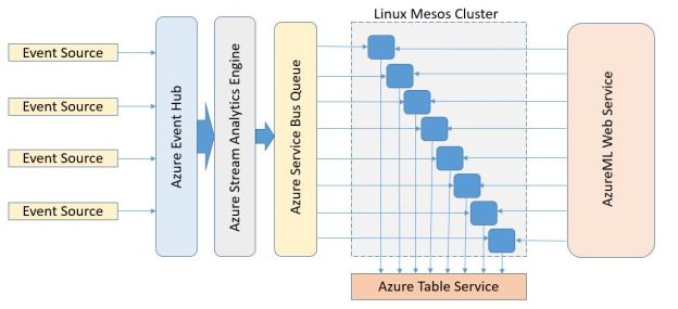
In this new version described here I want to see what sort of performance I could get from AzureML and Azure Stream Analytics.   To accomplish this goal I set up the pipeline shown in Figure 1.

system-diagram-eventhub

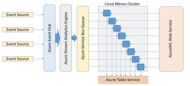
Figure 1.   Stream event pipeline

As shown in the diagram events (document abstracts) are initially pushed into the event hub which is configured as the source for the stream analytics engine.  The analytics engine does some initial processing of the data and then pushes the events to a message queue in the Azure Message Bus.  The events are then pulled from the queue by a collection of simple microservices which call the AzureML classifier and then push the result of the call into the azure table service.

In the following paragraphs I will describe how each stage of this pipeline was configured and I will conclude with some rather surprising throughput results.

Pushing events into the Event Hub.

To get the events into the Event Hub we use a modified version the solution posted by Olaf Loogman.  Loogman’s post provides an excellent discussion of how to get an event stream from the Arduino Yun and the Azure event hub using a bit of C and Python code.  Unfortunately the Python code does not work with the most current release of the Python Azure SDK[1], but it works fine with the old one. In our case all that we needed to do was modify Loogman’s code to read our ArXiv RSS feed data and convert it into a simple JSON object form

{ ‘doc’: ‘the body of the paper abstract’,
  ‘class’: ‘one of classes:Physics, math, compsci, bio, finance’,
  ‘title’: ‘ the title of the paper’ 
  }

The Python JSON encoder is very picky so it is necessary to clean a lot of special characters out of the abstracts and titles.  Once that is done it is easy to push the stream of documents to the Event Hub[2].

According to Microsoft, the Event Hub is capable of consuming many millions of events per second.  My simple Python publisher was only able to push about 4 events per second to the hub, but by running four publisher instances I was up to 16 eps.   It was clear to me that it would scale to whatever I needed.

The Stream Analytics Engine

The Azure stream analytics engine, which is a product version of the Trill research project, has a very powerful engine for doing on-line stream processing.   There are three things you must do to configure the analytics engine for your application.    First you must tell it where to get its input.   There are three basic choices:  the event hub,  blob storage and the “IOT” hub.   I configured it to pull from my event hub channel.   The second task is to tell the engine where to put the output.  Here you have more choices.  The output can go to a message queue, a message topic, blob or table storage or a SQL database.  I directed it to a message queue.  The final thing you must do is configure the query processing step you wish the engine to do.   For the performance tests described here I use the most basic query which simply passes the data from the event hub directly to the message queue.   The T-SQL code for this is

SELECT 
     *
INTO
     eventtoqueue
FROM
     streampuller

where eventtoqueue is the alias for my message bus queue endpoint and streampuller is the alias for my event queue endpoint.  The original JSON object that went into the event hub emerges with top level objects which include the times stamps of the event entry and exit as shown below.

{  "doc": "body of the abstract",
   "class": "Physics",
   "title":"title of the paper",
   "EventProcessedUtcTime":"2015-12-05T20:27:07.9101726Z",
    "PartitionId":10, 
    "EventEnqueuedUtcTime":"2015-12-05T20:27:07.7660000Z"
}

The real power of the Analytics Engine is not being used in our example but we could have done some interesting things with it.   For example, if we wanted to focus our analysis only on the Biology documents in the stream, that would only require a trivial change to the query.

SELECT
     *
INTO
    eventtoqueue
FROM
    streampuller
    WHERE class = ‘bio’

Or we could create a tumbling window and group select events together for processing as a block.  (I will return to this later.) To learn more about the Azure Analytics Engine and T-SQL a good tutorial is a real-time fraud detection example.

Pulling events from the queue and invoking the AzureML service

To get the document events from the message queue so that we can push them to the AzureML document classifier we need to write a small microservice to do this.  The code is relatively straightforward, but a bit messy because it involves converting the object format from the text received from the message queue to extract the JSON object which is then converted to the list form required by the AzureML service.   The response is then encoded in a form that can be stored in the table.    All of this must be encapsulated in the appropriate level of error handling.   The main loop is shown below and the full code is provided in Github.

def processevents(table_service, hostname, bus_service, url, api_key):
    while True:
       try:
            msg = bus_service.receive_queue_message('tasks', peek_lock=False)
            t = msg.body
            #the message will be text containing a string with a json object 
            #if no json object it is an error.  Look for the start of the object
            start =t.find("{")
            if start > 0:   
                t = t[start:]
                jt = json.loads(t)
                title = jt["title"].encode("ascii","ignore")
                doc  = jt["doc"].encode("ascii","ignore") 
                tclass = jt["class"].encode("ascii","ignore")
                evtime = jt["EventEnqueuedUtcTime"].encode("ascii", "ignore")
                datalist = [tclass, doc, title]
                #send the datalist object to the AzureML classifier
                try:
                       x = sendrequest(datalist, url, api_key)
                       #returned value is the best guess and 
                       #2nd best guess for the class
                       best = x[0][1]
                       second = x[0][2]
                       #save the result in an Azure Table using the hash 
                       # of the title as the rowkey
                       #and the hostname of this container as the table partition
                       rk = hash(title)
                       timstamp = str(int(time.time())%10000000)
                      item = {'PartitionKey': hostname, 'RowKey': str(rk),
                              'class':tclass, 'bestguess':best, 'secondguess':second,
                              'title': title, 'timestamp': timstamp, 'enqueued': evtime}
                      table_service.insert_entity('scimlevents', item)
                 except:
                        print "failed azureml call or table service error"
           else:
                 print "invalid message from the bus"
       except:
          print "message queue error”

Performance results

Now that we have this pipeline the most interesting experiment is to see how well it will perform when we push a big stream of messages to it.

To push the throughput of the entire pipeline as high as possible we wanted as many instances of the microservice event puller as possible.   So I deployed a Mesos Cluster with 8 dual core worker nodes and one manager node using the template provided  here.   To maximize parallelism for the AzureML service, three additional endpoints were created.   The microservices were assigned one of the four AzureML service endpoints as evenly as possible.

We will measure the throughput in seconds per event or, more accurately, the average interval between event arrivals over a sliding window of 20 events.     The chart below shows the seconds/event as the sliding window proceeds from the start of a stream to the end.   The results were a bit surprising.   The blue line represents one instance of the microservice and one input stream.   As you can see there is a very slow startup and the performance levels out at about 1 second/event.   The orange line is the performance with 12 microservice instances and four concurrent input streams.  Again the startup was slow but the performance leveled off at about 4 events/sec.

stream2

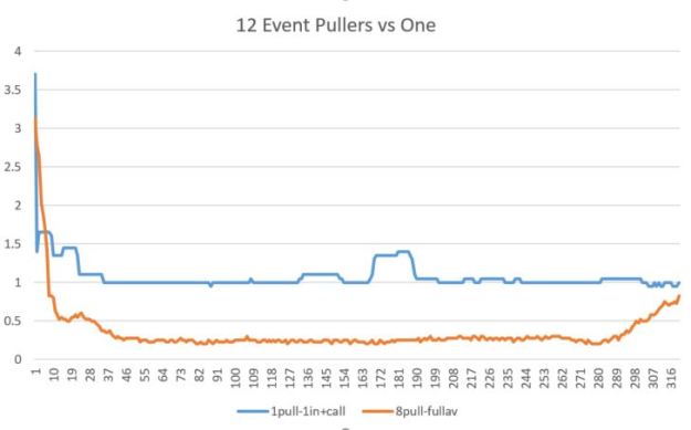
Figure 2.   Performance in Seconds/Event with a sliding window of 20 events.   Event number on the x-axis.

This raises two questions.

  1. Why the slow startup?
  2. Why the low performance for 12 instance case? Where is the bottleneck in the pipeline? Is it with the Azure Stream Analytics service,  the message bus or the AzureML service?

Regarding the slow startup, I believe that the performance of the Azure services are scaled on demand.  In other words, as a stream arrives at the event hub, resources are allocated to try to match the processing rate with the event arrival rate.   For the first events the latency of the system is very large (it can be tens of seconds), but as the pool of unprocessed events grows in size the latency between event processing drops very fast.   However, as the pool of unprocessed events grows smaller small resources are withdrawn and the latency goes back up again.  (We pushed all the events into the event hub in the first minute of processing, so after that point the number in the hub declines.  You can see the effect of this in the tail of the orange curve in Figure 2.)  Of course, belief is not science.   It is conjecture.

Now to find the bottleneck that is limiting performance.   It is clear that some resources are not scaling to a level that will allow us to achieve more than 4 events/second with the current configuration.   So I tried two experiments.

  1. Run the data stream through the event hub, message bus to the microservices but do not call the AzureML service.   Compare that to the version where the AzureML service is called.
  2. Run the data stream directly into the message bus and do not call the AzureML service.  Compare that one to the others.

The table below in Figure 3 refers to experiment 1.   As you can see, the cost of the AzureML service is lost in the noise.   For experiment 2 we see that the performance of the message bus alone was slightly worse that the message bus plus the eventhub and stream analytics.  However, I expect these slight differences are not statistically significant.

stream3

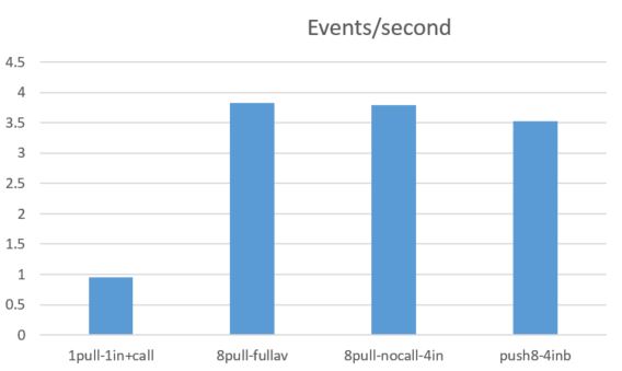
 Figure 3.  Average events per second compairing one microservice instance and one input stream to 8 microservices and 4 input streams to 8 microservices and 4 input streams with no call to AzureML and 8 microservices with 4 input streams and bypassing the eventhub and stream analytics.

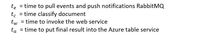
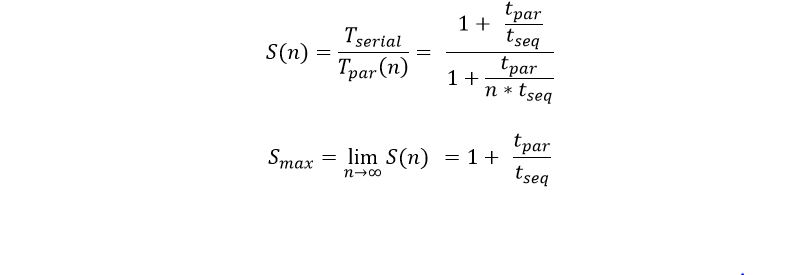
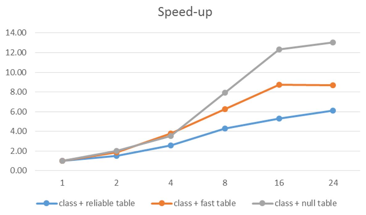
The bottom line is that the message bus is the bottleneck in the performance of our pipeline.  If we want to ask the question how well the AzureML service scales independent of the message bus, we can replace it with the RabbitML AMQP server we have used in previous experiments.     In this case we see a very different result.   Our AzureML service demonstrates nearly linear speed-up in terms of events/sec.    The test used an ancreasing number of microservices (1, 2, 4, 8, 12, 16 and 20) and four endpoints to the AzureML service.   As can be seen in Figure 4 the performance improvement lessens when the number of microservice instances goes beyond 16.  This is not surprising as there are only 8 servers running all 20 instances and there will be contention over shared resources such as the network interface.

stream4

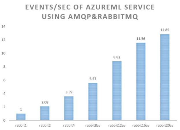
Figure 4.   AzureML events per second using multiple microservice instances pulling the event stream from a RabbitMQ server instance running on a Linux server on Azure.

Takeaway

It was relatively easy to build a complete event analytics pipeline using the Azure EventHub, Azure Stream Analytics and to build a set of simple microservices that pull events from the message bus and invoke an AzureML service.   Tests of the scalability of the service demonstrated that performance is limited by the performance of the Azure message bus.    The AzureML service scaled very well when tested separately.

Because the Azure services seems to deliver performance based on demand (the greater the number unprocessed events in the EventHub, the greater the amount of resources that are provisioned to handle the load.)  The result is a slow start but a steady improvement in response until a steady state is reached.   When the unprocessed event pool starts to diminish the resources seem to be withdrawn and the processing latency grows.      It is possible that the limits that I experience were because the volume of the event stream I generated was not great enough to warrant the resources to push the performance beyond 4 events/sec.   It will require more experimentation to test that hypothesis.

It should also be noted that there are many other ways to scale these systems.  For example, more message bus queues and multiple instances of the AzureML server.    The EventHub is designed to ingest millions of events per second and the stream analytics should be able to support that.  A good practice may be to use the Stream Analytics engine to filter the events or group events in a window into a single block which is easier to handle on the service side.   The AzureML server has a block input mode which is capable of processing over 200 of our classification events per second, so it should be possible to scale the performance of the pipeline up a great deal.


[1] The Microsoft Azure Python folks seem to have changed the namespaces around for the Azure SDK.   I am sure it is fairly easy to sort this out, but I just used the old version.

[2] The source code is “run_sciml_to_event_hub.py” in GitHub for those interested in the little details.

Performance Analysis of a Cloud Microservice-based ML Classifier

(This is an edited version correcting some of the analysis in the version i posted last week)

Microservice architectures have become an important tool for large scale cloud application deployment. I wanted to understand how well a swarm of microservices could be used to process streams of events where a non-trivial computation is required for each.   I decided a fun test would be to use machine learning to classify scientific document abstract that appear on public RSS feeds.   This is the first result of that experiment.  It uses a very small Mesosphere cluster on Microsoft Azure.   I will release the code to GitHub and data as soon as i clean it up a bit.

In a previous post we looked at building a document classifier for scientific paper abstracts.   In this post we will see how we can deploy it as a network of containerized microservices running on Mesosphere on Microsoft Azure.  We will then push this network of services hard to see how well it scales and we will try to isolate the performance issues. Specifically we are interested in the following challenge. If you have a heavy stream of events coming into a stream analysis system you may overload your services.   The conventional wisdom is that you can scale up the number of servers and services to cope with the load.   Fortunately more than one microservice instance can be deployed on a single VM. But does increasing the number of services instances per VM allow us to scale the system to meet the throughput requirements? Are there fundamental limits to how well this strategy will work? What are the limiting factors?

To summarize where we are so far, we have a set of RSS feeds that are “pushing” scientific publication events to us.   Our system looks at the abstracts of these events and use several different machine learning tools to classify the document into one (or more) scientific disciplines and sub-disciplines.   We have five major disciplines: Physics, Math, Biology, Computer Science and Finance. Each of these major disciplines is further divided into a number of sub-disciplines or specialties. We have divided the work into four main activities

  1. Training the classifiers. For this we used some of the labeled data from the ArXiv RSS feeds as training data.   (This was discussed in detail in the previous post, so we won’t go over it again here.)   This training phase is used to generate models that will be used by the classifier services discussed here.   We generate models for the main topic classifier and each of the sub-domain classifiers.   This is a pre-processing step and it is not counted in our performance analysis.
  2. Pulling the events from the RSS feeds and pushing them to the main topic classifier. The main topic predictor/classifier uses two primary machine learning methods to determine which disciplines the incoming documents belongs to.   As we have seen, these two methods agree on the discipline about 87% of the time. But sometimes they disagree on a document and we have two potential correct answers.   We interpret this as a potentially “interdisciplinary” research document and classify it as belong to both answers.
  3. Doing the sub-domain classification. As shown in the Figure 1 below the major topic classifiers push the document to the one (or two) sub-discipline specific classifiers.   These classifiers use the same ML methods as the main topic classifier to further classify the document into the sub-disciplines.

architecture

Figure 1.   Conceptual model of the document classifier microservice architecture

Managing queues and Pushing the classified document to a table of results.

What is not shown in the diagram in Figure 1 is what happens next. While the conceptual model provides a reasonable top-level view, the real design requires several additional critical components.   First as events move through the system you need a way to buffer them in queues.   We use the Active Message Queuing Protocol (AMQP) which is one of the standards in this space.   A good implementation of AMQP is the RabbitMQ system which we hosted on a server in the Azure cloud.     As shown in Figure 2   we (logically) position the RabbitMQ event hub between the major topic classifiers and the sub-domain classifiers.   We establish 7 queues on the event hub.   There is a queue for each of the major topic areas (Physics, Bio, Math, CS, and Finance), a “status” queue and a “role” queue.   The classify microservices are given classification roles by polling the “role” queue.   This tells them which topic area they are assigned to.   When they complete the sub-domain classification of a document they invoke another microservice that is responsible for storing the result in the appropriate table partition for later lookup by the users. This microservice sends an acknowledgement of the completed classification back to the event “status” queue prior. We shall refer to this microservice as the Table Web Service.  The “Status Monitor” is the overall system log and is critical for our performance measurements.

arch-detail

Figure 2.   The detailed architecture picture.

The Execution Environment

The RabbitMQ server is hosted on a Linux VM on Microsoft Azure and the rest of the system is deployed on a small Mesosphere cluster in a different Azure data center (see Figure 3).   The cluster is indeed small. There is one master node that runs the Mesosphere life cycle management services, the web browser interface and Marathon job management service. There are 5 dual core worker VMs. The Azure table is also a separate service.   The experiment status monitor runs in an IPython Notebook on my laptop.  experiment-setup

Figure 3.  Execution Environment

Using the web interface for Marathon we deploy different service configurations for the experiments described here.   Our table-pusher web service listens on a fixed port, so we can only have one instance per worker VM.   In practice this works out reasonably well because the classify services on any VM can invoke the local copy with very little overhead.   However, as we shall see, there are other major overheads associated with this service that will play a large role in the performance analysis.

We are not limited by the number of classify services we deploy.   If the system operator wants 20 “physics” sub-domain classifiers, the operator need only increase the deployment size of the classifier service by 20 and then submit 20 “physics” role messages into the role queue.

The Microservice Life Cycles

The top-level topic classifiers take the data from the RSS streams and apply the machine learning algorithms to produce the best 1 (or 2) potential topics.   The result is converted to a json object which contains

  1. The domain as determined by the random forest classifier we call RF
  2. The domain as determined by a hybrid classifier we call “the best of 3 classifier” (see the previous post) we call Best.
  3. The title of the document
  4. The body (abstract) of the document.

This doc json object is then pushed into the queue specified by the ML classifiers. If both RF and Best agree on a topic like “math” then the document is put in the “math” queue.   If they disagree and one says “math” and the other says “bio” then the document is placed in both the “math” and “bio” queues.    The classifier microservice has the following life-cycle.

ML Classifier

  1. When launched it opens a connection to the “roles” queue and wait for a topic.
  2. When it receives the topic message from the “role” queue the classifier service, must initialize all the ML models for that topic from the saved trained models. (The models have been previously trained as described in the previous post and the trained models have been “pickled” and saved as blob in Azure blob storage.)
  3. It then begins to scan the queue for that topic.   It pulls the json document objects from the queue and applies the classifier. It then packages up a new json object consisting of the main topic, new sub-classification, title and abstract. For example, if the item came from the “physics” queue and the classifier decides it in the subclass “General Relativity”, then that is the sub-classification that in the object. (The classifier also has a crude confidence estimator. If it is not very certain the sub-classification is “General Relativity?”.   If it is very uncertain and General Relativity is the best of the bad choices, then it is “General Relativity???”.) It then sends this object via a web service call to a local web service (described below) that is responsible for putting the object into an Azure table. (more on this step below. )
  4. The service repeats 3 until it receives a “reset” message in the topic queue.   It then returns to the roles queue and step 1.

Table Web Service

(note: this is a revised version.   the reliable and fast versions were incorrectly described in the  previous version of this post.)

The table web service is the microservice component that receives web service invocations from the classifier. Staying true to the Microservice design concept it has only one job.

  1. When Invoked it pulls the json object from the invocation payload and formats a Table service tuple to insert into the partition of the table associated with the main topic.
  2. We actually have three versions of web service one we call “fast” and the other “reliable” and the other is “null”.
    • The “reliable” version works by making a new connection to the RabbitMQ event server and then opens a channel to send it messages.  It then inserts the tuple in  table and then sends a time stamped status notification to  the event queue.
    • The “fast” version reuses the RabbitMQ connection for as long as possible. For each invocation it opens the channel and inserts the message.
    • The “null” version skips the Azure table entirely and is used only for the performance evaluation.

(Unfortunately, the RabbitMQ connection will timeout if there is a lull in the use and catching the timeout connection and restarting it proved to be problematic.   So the “fast” version is only used to illustrate the performance models below. It is not reliable. The “reliable” version is very reliable.   It runs for months at a time without problems. As we shall see, it is slower.  The “null” version is fast and reliable but not actually useful for anything other than benchmarks.)

  1. Before returning a web service response to the calling classifier instance the web-service sends a time-stamped message to status queue.

The Experiment

It was stated at the outset of this document that we are interested in understanding the effect of scaling the number Docker containers on the ability of the system to meet the flow of events into the system. To test the system under load we pre-loaded 200 abstract for the Biology topic into the message queue and all the classifier service instances were instructed to be Biology sub-topic classifiers.   We then ran this with 1, 2, 4, 8, 16 and 24 instances of the classifier microservice.   We ran this against all three versions of the table web service.   To compute the elapsed time to consume and process all 200 abstracts the table web service appended a timestamp to each status message. By looking at the time stamp for the first message and the last message we could determine the system throughput. (There were five different worker VMs so there is a small issue of clock skew between timestamps, but this was negligible.   What was not negligible was delays cause by network traffic between the data centers.   Hence I would estimate that the error bars for all the number below to be about 10%. We ran many tests and the number below are averages.

The most important number is the throughput of the system in classifications per second.   The table in Figure 4 summarizes the results.   Clearly the best throughput was obtained with the combination of the null classifier and the null table service.   The next best was the combination of the classifier and the null table service.

throughput

Figure 4. Throughput results for 1, 2, 4, 8, 16 and 24 instances of the classifier service.

The combination of the classifier and either the fast or reliable table service showed rather poor performance.   To understand this we need to look at the basic flow of execution of a single classifier and a single table web service as shown in Figure 5.   Note that the classifier that invokes the web service cannot return to fetch another task until the table web service has sent the status message.

classify-thread

Figure 5. Flow of control of the classify-table web service from the message queue and back.

To understand where congestion may exist look at the points where resource contention may occur when multiple classify instances are running.   This is illustrated in Figure 6.

classify-pipeline

Figure 6.   The major points of resource contention occur when the services access the Azure Table service and the RabbitMQ message broker.

Quantifying this let

eq1 - Copy

We can do a very crude speedup analysis based on Amdahl’s law.   Looking at the part of the computation that is purely parallel and assuming sequential access to the Table service and message broker we can say

eq2 - Copy

tseq is a function of the two points of contention.   It turns out that the message queue is fast in comparison to the Azure table service.   This is due to the complexity of inserting an item into a table. Because we are only using one table partition “Biology” all our inserts go into one place.   Unfortunately, inserts into any disk-based system are going to involve locks so this is not surprising.  However, the difference between the fast version and the reliable version illustrate the high cost of establishing a new connection to the message broker for each event.  I am not sure what the function “f” is above but i suspect it is additive.

Let Tserial be the time for one instance of the classify service to complete the execution the set of messages and Tpar (n) be the time it takes n instances to do the job. We then have

eq3 - Copy

The speedup of n classifiers over a single classifier is then

eq4 - Copy

Analysis of the data on the time to do a single classifier with no table service give us tpar = 450 ms (approximately) and tseq  = 60 ms for the fast service and 100 ms for the reliable service.   Using the formula above we have the maximum speed-up Smax   = 8.5 for the fast service an 5.5 for the reliable service.   This approximately agrees with the results we can measure as seen in figure 7 below.

speedup

Figure 7.   Speed-up relative to one instance of the classifier with different table services plotted against different numbers of classifier instances.

Of course speed-up is a relative number, but it does illustrate the way systems scale.   As we can see the limits are approximately what we predicted.   However the case of the null table is different.   There should be essentially no sequential component so why is it flat-lining at around 13? The answer is that there are only 10 cores in our system.   That puts a fundamental limit on the performance.   In fact we are lucky to get more than a speed-up of 10.

Conclusions

One thing that does not come out in the text above is how well the concept of microservices worked.   One of the major selling points for this style of application construction is that factoring of the services into small independent components can help with maintenance of the overall system.   Using Mesosphere and the Marathon task scheduled proved this point well.   It was possible to modify, remove and scale any of the services without having to bring down the others.   This made all of the experiment described above easy to carry out.   And the system remained up for several months.

It is clear that 10 cores is not a very impressive platform to test scalability.   We did demonstrate that we could easily scale to about 2.5 services per core without problems.   Going beyond that did not improve performance.   I am currently trying to build an instance of Mesosphere or other Docker cluster mechanism (perhaps Swarm) with at least 100 servers.   I will update these results when i have that complete.

Another thing to do is cache the table writes and then update the table with an entire block.   A good solution for this is to introduce a Redis cache service.   Fortunately Docker makes this trivial.   Redis containers are  in the library.  Doing this and having a much larger cluster should enable at least a 20x improvement.

Actually, a more interesting experiment is to try this classification problem using one of the more conventional tools that already exist.   For example Microsoft Stream Analytics + Azure Machine Learning & Microsoft StreamInsight, Spark Streaming + Event Hubs and HDInsight, Amazon Kinesis, Google BigQuery, IBM Watson Analytics and numerous open source IoT platforms.   I plan to start with the Azure solution while i still have Azure resources.

I am in the process of moving all the code and data for this experiment into GitHub.   I will post link to these items in the next week or so.