Building a “ChatBot” for Scientific Research

We can use Alexa, Cortana and Siri to check the weather, stream our favorite music and lookup facts like “who directed Casablanca?” But if I want to find all the research on quantum entanglement in the design of topological quantum computers, these services will fall short.   If, in addition, I want these articles cataloged in my personal archive and the citations automatically pulled I need a much more robust digital assistant.  Raj Reddy talks about a broader and more pervasive future for digital assistant he calls Cognition Amplifiers and Guardian Angels.  In this post we look at chatbots and their limitations and show how to build a simple, voice-driven scientific metasearch tool we call the research assistant.  Finally, we discuss the next phase of research assistant.

Smart Speakers and Chatbots.

The revolution in “smart speaker” digital assistants like Siri, Amazon Echo, Google Home is showing us the power of voice to provide input to smart cloud services.   These assistants can take notes, tell us the weather conditions, place on-line orders for us and much more.   I even allow Microsoft’s Cortana to read my email.  If I send the message “I’ll get back to you tomorrow” to a friend, Cortana will remind me the next day that a response is needed.  Amazon allows people to add “skill” (additional capabilities) to there Alexa system.  These smart speakers are designed around open-ended question-response scenario.  These assistants leverage very powerful speech-to-text technology and semantic analysis systems to extract a query or command.  The query answers are derived from web-data analysis and the commands are to a limited number of native services (or external skills).

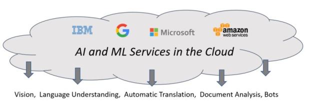
A chatbot is a system that engages the user in a dialog.   They go beyond the question answering smart speakers and are usually designed to help people interact with the services of a specific company or agency.   The Google, IBM, Amazon and Microsoft have all introduced cloud services to help anybody build a chatbot.   These services guide you through the process of building and training a chatbot.   A good example is Google’s Dialogflow.   Using this tool to create a bot, you specify three things:

  • Intents – which are mapping between what the user says and how you wish the system to respond.
  • Entities – that are the categories of subjects that your bot understands. For example, if you bot is a front end to your clothing store, one category of entity my be product type: shoes, dress, pants, hats,  and another entity might be size: large, xl, small, medium,  and another might be color.
  • Context – This is knowledge obtained by the bot during the course of the conversation. For example, the name of the user, or the users favorite shoe color.

The goal of the bot is to extract enough information from the user to take a meaning action such as fulfilling an order.   The hard part is designing the intents so that a dialog can lead to the desired conclusion.  The resulting sysgtem is called an agent and the flow of action is illustrated in Figure 1.  It might start with ‘Good morning, how can I help you?’   and end with a summary of the discussion.  As the programmer you need to supply as many possible variations on possible user questions and responses as possible.  And you must annotate these with makers where your entities can be extracted.    Your examples are used in a training phase that maps your intents and entities together and builds a model that will learn variations on the input and not repeat the same sequence of responses each time, so it seems less robotic to the user.

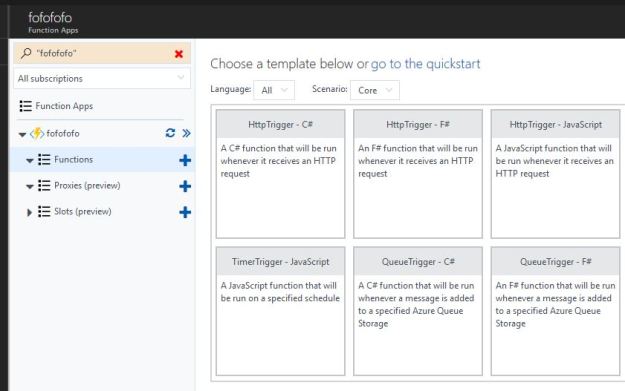
Amazon’s Lex provides a similar service that also integrates with their lambda services.  Microsoft has the Azure Bot Service and IBM has Watson assistant chatbot tools.

dialogflow

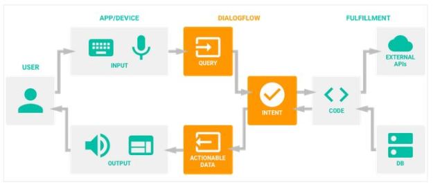
Figure 1. Google Dialogflow Agent architecture.

These tools are all designed to help you build a very focused conversation with the user about a very narrow universe such as the on-line part of a business.   But this raises the question, can one build a chat bot that can carry out an open-ended conversation.  Perhaps one that could pass the Turing test?   The research literature on the subject is growing and deep learning tools like recurrent and convolutional neural networks have been applied to the problem (see https://arxiv.org/pdf/1606.07056.pdf , https://arxiv.org/pdf/1605.05110.pdf and more).   Unfortunately chatbots designed to engage in open-ended conversation have only had a limited success.   Xiaoice is one that interacts with users on the Chinese micro blogging service Weibo.  The problem is that while it sounds like conversation, it is mindless.  Microsoft’s Tay was an English language version that operated on Twitter until it was taken down after only 16 hours because of the unfortunate language it had learned.  A successor Zo seems to be working better, but it does not produce conversations with intellectual content.

There is an excellent pair of articles by Denny Britz about the role of deep learning for conversational assistants.   He make the point that for open-ended conversations (he calls them open-domain) the challenges are large compared to the fixed domain chatbots because so much more world knowledge is required.

Cognition Amplifiers and the Research Assistant.

In the spring of 2018 Raj Reddy gave the keynote presentation at the IEEE services congress.  His topic was one he has addressed before and it clearly resonated with the audience.   He described Cognition Amplifiers and Guardian Angels.  He defined a Cognition Amplifier (COG) as a Personal Enduring Autonomic Intelligent Agent that anticipates what you want to do and help you to do it with less effort. A Guardian Angel (GAT) is a Personal Enduring Autonomic Intelligent Agent that discovers and warns you about unanticipated events that could impact your safety, security and happiness.

Consider now the application of the Cognition Amplifier to scientific research.   If you are working on writing a research paper, you may wish your autonomic research assistant to provide a fast and accurate search of the scientific literature for a specific list of scientific concepts. In fact, as you write the paper, the assistant should be able to pick up the key concepts or issues and provide a real-time bibliography of related papers and these should be stored  and indexed in a private space on the cloud.  Extracting key phrases from technical documents is already a heavily research field so applying this technology to this problem is not a great leap.   However, key phrase extraction is not the whole challenge.   Take sentence “It seems that these days investors put a higher value on growth than they do on profitability”.  The categorical topic is value of growth vs profitability – investor opinions which is not simply a key phrase, but a concept and we need the research assistant to look for concepts.    Your research assistant should always understand and track the context of your projects.

Finally, a good research assistant for science should be able to help with the analytical part of science.  For example, it should help locate public data in the cloud related to experiments involving your topics of interest.   The assistant should be able to help formulate, launch and monitor data analysis workflows. Then coordinate and catalog the results.

And, of course, if your autonomous research assistant is also a Guardian Angel, it will also keep you informed of grant reporting deadlines and perhaps pull together a draft quarterly report for your funding agency.

I fully expect that it is possible to build such an agent in the years ahead.   However, the remainder of this article is a simple demo that is a far cry from the full research assistant agent described above.

The Research Assistant Metasearch Tool.

In the following paragraphs we describe a very simple voice-driven agent that can be used to look for research articles about scientific topics.  We also show how such a system can be assembled from various simple devices and cloud services.   The system we describe is not very sophisticated.  In fact it is not much better than Cortana at finding things given English input sentence.  However we feel it does illustrate the architecture of a voice-driven agent that can be built by gluing together easy to use cloud services.

Our scenario is a researcher sitting near the device and asking about very specific research topics such as “physical models of immune response” or “programming a topological quantum computer”.    We assume the user wants a spoken response if that response is simple, but we also realize that this is impractical if the system is creating a list research journal papers.  To address this issue, the system also has a display in a web browser.  (We note that the Cortana and Google assistant do the same if the response is a list.)

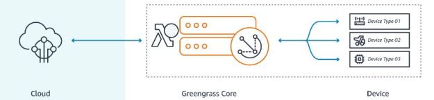
Figure 2 illustrates the basic architecture of the system.

architectureofRA

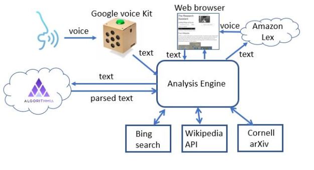
Figure 2.  The architecture of the research assistant.

The components of the system are:

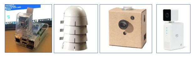
  1. The voice-to-text translator. Here we use a simple voice kit from google.   This consists of some special hardware and a raspberry pi 2 computer all packaged in an elegant cardboard box.  You wake the system up by pressing the botton on top and speak.   The audio is captured and sent to the google voice service for transcription and it is returned as a text string.
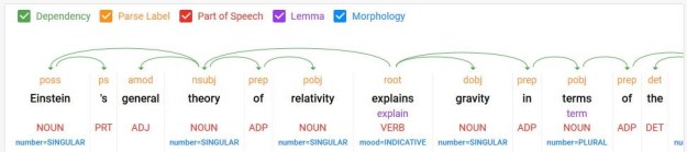
  2. The next step is to parse the text string into the components that will allow us to extract the topics of the query.  This is another cloud service call.  This time it is to Algorithmia.com and the service is called key phrases.  (we wrote about this in a previous article.)  The service takes English sentences and invoked Googles ParsyMcParseface (another Algorithmia.com AI service) and returns a list composed of three types of phrases: subject (s), actions (a) and objects (o).  It also flags prepositional phrases with a “/” character.   So for example, “I am interested in physical models of immune response” returns

          [‘s: I ‘, ‘a: am ‘,  ‘o: interested /in physical models /of immune response.’]

  1. The analysis engine is a 500-line Python Dash-based web server that extracts the topics and a few other items of interest and decides how to search and display the results on the browser. There are three web services used for the search: Wikipedia,  Bing and Cornell’s ArXiv service[1].  To see how this works, consider the example the sentence “research papers by Michael Eichmair about the gannon-lee singularity are of interest“. The analysis engine detects the topic as the gannon-lee singularity and Michael Eichmar as the author.  The fact that research papers are of interest indicates that the we should look in the Cornell ArXiv repository of papers.   (The results for this query are at the end of this section).    (Truth in advertising: our parser and analysis are far from perfect.   For example, “tell me about Deep Learning”   vs “tell me about deep learning” yield two different parses.  The first yields

            [‘a: tell ‘, ‘o: me /about Deep Learning ‘]

           which is fine. But the second gives us

          [‘a: tell ‘, ‘o: me about deep ‘, ‘a: learning ‘]

           which causes the analysis to fail. )

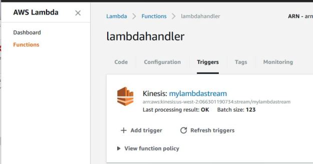
  1. Finally, we use the Amazon Lex services to generate the audio reading of the Wikipedia results. If you have an aws account, the Python API is easy to use.

Examples

Figure 3 illustrates the interface.  We have started with the statement “I am interested in physical models of immune response.”

fig3-chatbot

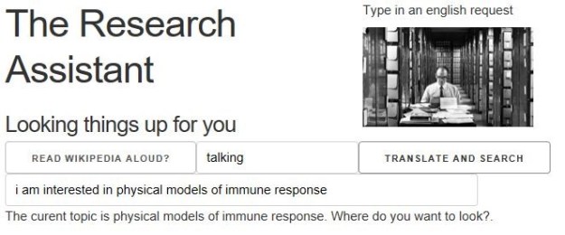
Figure 3.   The interface provides a switch to allow the Wikipedia response to read aloud.   In this case we have typed the English statement of intent into the query box and hit the “Translate and Search” button.

We respond with the phrase “look for it in Wikipedia” and get the result in figure 4.    Following that response, we say “how about research papers” and we get the response in figure 5.

webpage3

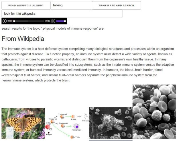
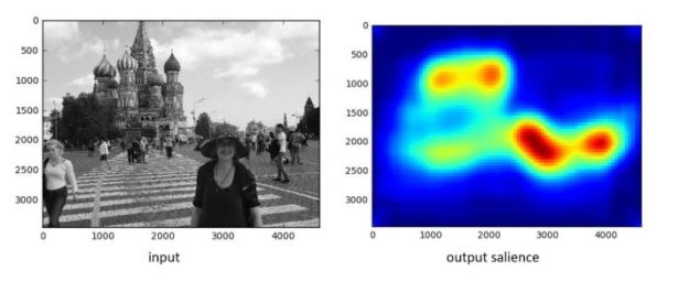
Figure 4.   The response to “look for it in wikipedia”.  A short summary from Wikipedia is extracted along with related images found on the subject.  The spoken response is controlled by the audio control  at the top of the response.

webpage4

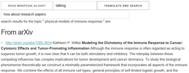
Figure5.   The mention of research papers suggest that we should consult the Cornell library arXiv.    Shown above is only the first result of 10 listed on the page.

Returning to the example mentioned above “research papers by Michael Eichmair about the gannon-lee singularity are of interest” we get the following results.   You will notice that the Wikipedia result is a default hit for “big bang singularity” and not directly related to the precise query.  The Bing results and the ArXiv hits are accurate.

webpage5

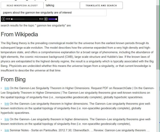
Figure 6.  Results for the query “research papers by Michael Eichmair about the gannon-lee singularity are of interest”.  (This page was slightly edited to shorten the list of Bing results.)

The system has a limited capability to pull together concepts that are distributed over multiple sentences.  For example the input string “what are anyons?   How do they relate to topological quantum computation?” will build the topic “anyons topological quantum computation”.

If you are interested in trying to use the system point your browser here.  I will try keep it up and running for a few months. There is no voice input because that requires a dedicated Google voice kit on your desk.   You need to decide if you want to have a playback of the audio for Wikipedia summaries.   If you don’t want it, simply press the “Read Aloud” button.  Then enter a query and press the “Translate and Search” button.   Here are some samples to try:

  1. what did they say about laughter in the 19th century?
  2. are there research papers about laughter by Sucheta Ghosh?
  3. what can you tell me about Quantum Entanglement research at Stanford? (this one fails!)
  4. what can you tell me about research on Quantum Entanglement at Stanford?
  5. what are anyons? How do they relate to topological quantum computation?
  6. Who was Winslow Homer? (this one give lots of images)
  7. I am interested in gravitational collapse. (respond with web, Wikipedia or arxiv)

As you experiment, you will find MANY errors.  This toy is easily confused.   Please email me examples that break it.  Of course, feedback and suggestions are always welcome.  I can make some of the source code available if there is interest. However, this is still too unreliable for public github.

[1] There are other arguably superior sources we would like to have used.  For example, Google Scholar would be perfect, but they have legal restrictions on invoking that service from an application like ours.  Dblp is also of interest but it is restricted to computer science.

The State of the Cloud for Science -2018

Introduction

This post is based on a talk I prepared for the Scientific Cloud Computing Workshop at HPDC 2018.

Two years ago, Ian Foster and I started writing  “Cloud Computing for Science and Engineering”.   That book covers fundamental cloud tools and computational models, but there are some topics we alluded to but did not explore fully because they were still on the horizon.  In other cases, we were simply clueless about changes that were coming. Data center design and cloud services have evolved in some amazing ways in just two years and many of these changes represent opportunities for using cloud technology in scientific research.

Whose cloud?

Any  discussion of cloud computing in science leads to the question of definition.  What defines a cloud for science?   For example, the European Open Science Cloud (EOSC) is a European-wide virtual environment for data sharing and collaboration.  That project will involve multiple data archives, research labs and HPC centers, commercial service providers and EU agencies and funding.  It is truly an important project.  However, my focus here is on the fundamental technologies that are driving hardware and software innovation, and these tend to come from a combination of academic, open source and commercial providers.   The most ubiquitous commercial clouds are:

  • Amazon Web Services (AWS) – 40% of all commercial cloud resources on the planet,
  • Microsoft Azure – about 50% of AWS but growing,
  • Google Cloud – a solid and growing third place,
  • IBM Bluemix – growing very fast and in some measures bigger now that Google.

There are many more, smaller or more specialized providers: Salesforce, DigitalOcean, Rackspace, 1&1, UpCloud, CityCloud, CloudSigma, CloudWatt, Aruba, CloudFerro, Orange, OVH, T-Systems.

There are a number of smaller cloud systems that have been deployed for scientific research.  They  include Aristotle, Bionimbus, Chameleon, RedCloud, indigo-datacloud, EU-Brazil Cloud,  and the NSF JetStream.  The advantage of these research clouds is that they can be optimized for use by a specific user community in ways not possible in a commercial cloud.  For example, Chameleon is funded by the US NSF to support basic computer systems research at the foundational level which is not possible when the foundation is proprietary.

Are these clouds of any value to Science?

When the first commercial clouds were introduced in 2008 the scientific community took interest and asked if there was value there.  In 2011 the official answer to this question seemed to be  “no”.  Two papers (see end node 1) described research experiments designed to address this question.   The conclusion of both papers was that these systems were no match for traditional supercomputers for running MPI-based simulation and modeling.   And, in 2010, they were correct.   Early cloud data centers were racks of off-the-shelf PCs and the networks had terrible bisection bandwidth and long latencies.   They were no match for a proper HPC cluster or supercomputer.

Over the last few years, others have recognized a different set of roles for the cloud in science that go beyond traditional supercomputer simulation.   The biology community was quick to adopt cloud computing especially when it is necessary to do large scale analysis on thousands of independent data samples.  These applications ranged from metagenomics to protein folding.   These computations could each fit on a single server, so network bandwidth is not an issue and, using the scale of the cloud, it is easy to launch thousands of these simultaneously.   Hosting and sharing large public scientific data collections is another important application.   Google, AWS, Microsoft and other have large collections and they also are also providing new ways to host services to explore this data.

However, there are at least three additional areas where the cloud is a great platform for science.

Analysis of streaming data

Microsoft’s AI for earth project (Figure 1) looks at the application of streaming data from sources such as satellites to do land cover analysis,  sensors on and above farm land to improve agriculture outcomes and crowd sourced data to help understand biodiversity.

urban0

Figure 1.  Applications of streaming include land cover analysis, using sensor data for improving agriculture and biodiversity.   From  https://www.microsoft.com/en-us/aiforearth

The internet of things is exploding with sensor data as are on-line experiments of all types.  This data will be aggregated in edge computing networks that do initial analysis with results fed  to the cloud systems for further analysis.   Urban Informatics is a topic that has emerged as critical to the survival of our cities and the people who live in them.  Sensors of all types are being deployed in cities to help understand traffic flow, microclimates, local pollution and energy waste.  Taken together this sensor data can paint a portrait of the city that planners can use to guide its future.  Streaming data and edge computing is a topic that will involve the growing capabilities and architecture of the cloud.  We will return to this later in this document.

Interactive big data exploration

Being able explore and interact with data is a critical component of science.   If it fits on our laptop we can use tools like Matlab, Excel or Mathematica to conduct small computational experiments and visualize the results.  If the data is too big it must be stored on something bigger than that laptop.   Traditional supercomputers are up to the task of doing the analysis, but because they are designed around batch computing there are not well suited to interactive use.   The cloud exists to host services that can be used by thousands of simultaneous users.   In addition, there is a new generation of interactive data analysis tools that are cloud-ready for use on very large data collections.  This collection of tools includes Spark and Python Dask.   In both cases these tools can be driven by the open-source Jupyter studio which provides a powerful, interactive compute and visualization tool.  The commercial providers have adapted Jupyter and its interactive computational model into their offerings.   Google has Cloud Datalab (Figure 2), Amazon uses Jupyter with its SageMaker Machine Learning platform and Microsoft provide a special data science virtual machine that runs Jupyter Hub so that teams of users can collaborate.

google-datalab

Figure 2.  Google’s Cloud Data lab integrates SQL-like queries to be combined with Python code and visualization to a Jupyter based web interface. https://cloud.google.com/datalab/

Being able to interact with data at scale is part of the power of the cloud.   As this capability is combined with advanced cloud hosted machine learning tools and other services, some very promising possibilities arise.

The quest for AI and an intelligent assistant for research

The commercial clouds were originally built to  host web search engines.   Improving those search engines led to a greater engagement of the tech companies with machine learning.   That work led to deep learning which enabled machine language translation,  remarkably strong spoken language recognition and generation and image analysis with object recognition.  Many of these  capabilities rival humans in accuracy and speed.  AI is now the holy grail for the tech industry.

One outcome of this has been the proliferation of voice-driven digital assistants such as Amazon’s Echo, Microsoft’s Cortana, Apple’s Siri and Google Assistant.   When first introduce these were novelties, but as they have improved their ability to give us local information, do web searching, keep our calendars has improved considerably.   I believe there is an opportunity for science here.

Ask the question “what would it take to make Alexa or Cortana help with my research?”   The following use cases come to mind.

  1. Provide a fast and accurate search of the scientific literature for a given specific scientific concept or topic and not just a keyword or specific author. Then ask who is working on or has worked on this topic?  Is there public data in the cloud related to experiments involving this topic?  Translate and transcribe related audio and video.
  2. Understand and track the context of your projects.
  3. Help formulate, launch and monitor data analysis workflows. Then coordinate and catalog results.  If state-space search is involved, automatically narrow the search based on promising findings.
  4. Coordinate meetings and results from collaborators.

If I ask Alexa to do any of this now, she would politely say “Sorry.  I can’t help you with that.”  But with the current rate of change in cloud AI tools, ten years seems like a reasonable timeframe.

siri-grandson

Figure 3.  Siri’s science geek grandson.

Technical Revolutions in the Cloud

Two of the three scenarios above are here now or very close.   The third is some ways off.   There have been three major changes in cloud technology in the past five years and some aspects of these changes are true game-changers for the industry.    The first, and most obvious is the change in scale of cloud deployments. The two leaders, AWS and Azure are planetary in scale.  This is illustrated in Figure 4 below.

cloud-scale

Figure 4.  A 2016 map of cloud coverage from Atomia.com.  https://www.atomia.com/2016/11/24/ comparing-the-geographical-coverage-of-aws-azure-and-google-cloud/ There is some inaccuracy here because AWS and Azure define regional data centers differently, so counting the dots is not a good comparison.   In addition, data centers are now under construction in South Africa and the Middle East.

This map does not include all the data centers run by the smaller cloud providers.

Cloud Services

A major departure from the early days of the cloud, where scientists focused on storage and servers, has been an explosion in pay-by-the-hour cloud hosted services.  In addition to basic IaaS the types of services available now are:

  • App services: Basic web hosting, mobile app backend
  • Streaming data: IoT data streams, web log streams, instruments
  • Security services: user authentication, delegation of authorization, privacy, etc.
  • Analytics: database, BI, app optimization, stream analytics
  • Integrative: networking, management services, automation

In addition, the hottest new services are AI machine learning services for mapping, image classification, voice-to-text and text-to-voice services and text semantic analysis.   Tools to build and train voice activated bots are also now widely available.   We will take a look at two examples.

A planet scale database

The Azure Cosmos DB is a database platform that is globally distributed.   Of course, distributing data across international boundaries is a sensitive topic, so the Cosmos platform allows the database creator to pick the exact locations you want copies to reside.   When you create an instance of the database you use a map of Azure data centers and select the locations as shown in Figure 5.

cosmos1

Figure 5.  Cosmos DB.  A database created in central US and replicated in Europe, South India and Brazil.

The database can support 4 modes: Documents, key-value Graph and NoSQL.  In addition, there are five different consistency models the user can select: eventual, consistent prefix, session, bounded stateless and strong consistency all with 99.9% guarantee of less than 15ms latency.  My own experiments validated many these claims.

Cloud AI Services

The commercial clouds are in a race to see who can provide the most interesting and useful AI services on their cloud platform.   This work began in the research laboratories in universities and companies over the past 25 years, but the big breakthroughs came when deep learning models trained on massive data collections began to reach levels of human accuracy.  For some time now, the public cloud companies have provided custom virtual machines that make it easy for technically sophisticated customers to use state of the art ML and neural network tools like TensorFlow, CNTK and others.  But the real competition is now to provide services for building smart applications that can be used by developers lacking advanced training in machine learning and AI. We now have speech recognition, language translation, image recognition capabilities that can be easily integrated into web and mobile applications.

We gave this a try with services that use a technique called Transfer Learning to make it possible to re-train a deep neural network to recognize objects from a narrow category using a very small training set.   We chose images of galaxies and used the services of IBM Watson, Azure and Amazon.   Figure 6 illustrates the results from IBM’s tool.  The results were surprisingly good.

galaxies

Figure 6.  IBM’s Watson recognizing previously unseen images of three different galaxies.  The details of this study are here: https://esciencegroup.com/2018/02/16/cloud-services-for-transfer-learning-on-deep-neural-networks/

The Revolution in Cloud Service Design

Making all of these services work, perform reliably and scale to thousands of concurrent users forced a revolution in cloud software design.    In order to support these applications, the tech companies needed a way to design them so that they could be scaled rapidly and updated easily.   They settled on a design pattern that based on the idea of breaking the applications into small stateless components with well defined interfaces.   Statelessness meant that a component could be replaced easily if it crashed or needed to be upgraded.   Of course, not everything can be stateless, so state is saved in cloud hosted databases.   Each component was a “microservice” and it could be built from containers or functions.  This design pattern is now referred to as “cloud native” design.   Applications built and managed this way include Netflix, Amazon, Facebook, Twitter, Google Docs, Azure CosmosDB, Azure Event hub, Cortana, Uber.

microservice
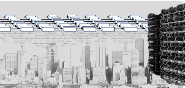
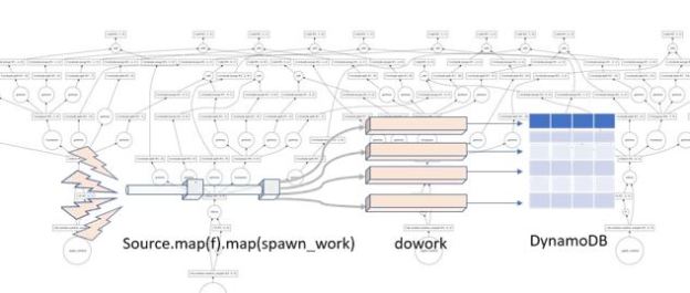
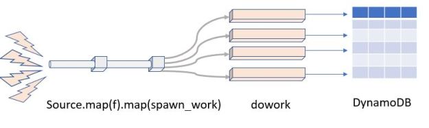
Figure 7.  Conceptual view of microservices as stateless services communicating with each other and saving needed state in distribute databases or tables.

To manage applications that required dozens to hundreds of concurrently running microservice you need a software foundation or container orchestration system to monitor the services and schedule them on available resources.  Several candidates emerged and are used. Siri, for example, is composed of thousands of microservices running on the Apache Mesos system.   Recently cloud providers have settled on a de-facto standard container orchestrator built by Google and released as open source called Kubernetes.   It is now extremely easy for any customer to use Kubernetes on many cloud deployments to launch and manage cloud native applications.

Serverless Functions

The next step in the cloud software evolution was the introduction of “serverless functions”.   The original idea of cloud computing involved launching and managing a virtual machine.  However, suppose you want to have a cloud-based application whose sole job is to wait for an event to trigger some action.  For example, monitor a file directory and wait for a change such as the addition of a new file.  When that happens, you want to send email to a set of users alerting them of the change.   If this is a rare event, you don’t want to have to pay for an idle virtual machine that is polling some service looking for a change.  Amazon was the first to introduce the concept of a function-as-a-service.   With AWS Lambda, you only need to describe the function in terms of the trigger event and the output actions it takes when the even appears.  As illustrated in Figure 8, there are many possible triggers and corresponding output channels.

lambda

Figure 8.   From Amazon AWS.   The triggers and outputs of a lambda function.

In addition to AWS Lambda, Azure Functions, Google Functions, IBM OpenWhisk are similar systems.  OpenWhisk is now open source.  Another open source solution is Kubeless that allow you to deploy a lambda-like system on top of your Kubernetes cluster.   These serverless systems let you scale up and down extremely rapidly and automatically.   You can have hundreds of instances responding to events at once.  And the cost is based on charge-by-use models.  AWS has  introduced AWS Fargate which allows any containerized application to run in serverless mode.

The Edge and the Fog

The frontier of cloud computing is now at the edge of the network.  This has long been the home of content distribution systems where content can be cached and access quickly, but now that the Internet-of-Things (IoT) is upon us, it is increasingly important to do some computing at the edge.  For example, if you have a thousand tiny sensors in a sensitive environment or farm and you need to control water from sprinklers or detect severe weather conditions, it is necessary to gather the data, do some analysis and signal an action.   If the sensors are all sending WIFI messages they may be routable to the cloud, but a more common solution is to provide local computing that can do some event preprocessing and response while forwarding summary data to the cloud.  That local computing is called the Edge, or if a distributed systems of edge servers, the Fog.

If serverless functions are designed to respond to signals, that suggests that it should be possible to extend them to run in the edge servers rather than the cloud.  AWS was the first to do this with a tool called GreenGrass that provides a special runtime system that allows us to push/migrate lambda functions or microservices from the data center to the edge.   More recently Microsoft has introduced Azure IoT Edge which is built on open container technologies.  Using an instance open source Virtual Kubelet deployed on the edge devices we can run our Kubernetes containers to run on the edge.  You can think of a Kubelet as the part of Kubernetes that runs on a single node. This enables Kubernetes clusters to span across the cloud and edge as illustrated in Figure 9.

edge-cloud

Figure 9.  shows a sketch of migrating containerized functions to edge function.   That way our IOT devices can communicate with locally deployed microservices.  These microservices can communicate with cloud-based services.  The edge function containers can also be updated and replaced remotely like any other microservice.

The Evolution of the Data Center

As mentioned at the beginning of this paper, the early days (2005) of cloud data center design systems were based on very simple server and networks were designed for outgoing internet traffic and not bisectional bandwidth for parallel computing.   However, by 2008 interest in performance began to grow.  Special InfiniBand sub-networks were being installed at some  data centers.  The conventional dual-core servers were being replaced by systems with up to 48 cores and multiple GPU accelerators.  By 2011 most of the commercial clouds and a few research clouds had replaced traditional network with software defined networking.  To  address the demand of some of its customers, in 2017 Microsoft added  Cray® XC™  and Cray CS™ supercomputers to a few data centers and then acquired the company cycle computing.

From 2016 we have seen progress focused on performance and parallelism.   The driver of this activity has been AI and, more specifically, the deep neural networks (DNNs) driving all the new services.  There are many types of DNNs but two of the most common are convolutional, which look like a linear sequence of special filters, and recurrent networks which, as the name implies, are networks with a feedback component.   And there are two phases to neural network design and use.  The first is the training phase which requires often massive parallelism and time.  But it is usually an off-line activity.  The second phase is called inference and it refers to the activity of evaluating the trained network on classification candidates.  In both the convolutional and recurrent network inference boils down to doing a very large number of matrix-vector and matrix-matrix multiplies where the coefficients of the matrix are the trained model and the vector represent the classification candidates.      To deliver the performance at scale that was needed by the AI services it was essential to do these operations fast.  While GPUs were good, more speed was needed.

Google’s Tensor Processing Unit

In 2015 Google introduced the Tensor Processing Unit (TPU) and the TPU2 in 2017.

google-tf1

google-tf2

Figure 10.  Above, Google data center.  https://www.nextplatform.com/2017/05/22/hood-googles-tpu2-machine-learning-clusters/  Below architecture of Google Tensor Processing Unit TPU. From “In-Datacenter Performance Analysis of a Tensor Processing Unit”, Norman P. Jouppi et al.​  ISCA 2017  https://ai.google/research/pubs/pub46078

Figure 10 illustrates several racks of TPU equipped servers and the functional diagram of the TPU.  One of the key components is the 8-bit matrix multiply capable of delivering 92 TeraOps/second (TOPS).   (It should be noted that DNNs can be well trained on less than IEEE standard floating-point standards and floating point systems with small mantissa are popular.)  The multiply unit uses a systolic algorithm like those proposed for VLSI chips in the 1980s.

Microsoft’s Brainwave

In 2011 a small team in Microsoft Research led by Doug Burger began looking at the use of FPGAs to accelerate the search result ranking produced by Bing.   Over several iterations they arrived at a remarkable design that allowed them to put the FPGA between the network and the NIC so that the FPGA could be configured into separate plane of computation that can be managed and used independently from the CPU (see Figure 11).   Used in this way groups of FPGAs could be configured into a subnetwork to handle tasks such as, database queries and  inference stage of deep learning in addition to Bing query  optimization.

brainwave0

Figure 11.  The Brainwave architecture.

brainwave

Figure 12. The brainwave software stack for mapping a DNN to one or more FPGAs. From BrainWave_HOTCHIPS2017.pptx, Eric Chung, et. al., https://vneetop.wordpress.com/ 2017/10/28/accelerating-persistent-neural-networks-at-datacenter-scale/

The team also built a software stack that could really make this possibility a reality.   What makes much of this possible is that the models for DNNs are all based on flow graphs which describe sequences of tensor operations.  As shown in Figure 12 above, the flow graphs can be compiled to a graph internal representation that can be split and partitioned across one or more FPGAs.  They refer to the result as a hardware microservice.   Just recently Mary Wall [see endnote 2] wrote a nice blog about the teams work on using this idea to do deep learning inference on land cover maps.  Each compiled inference hardware microservice is mapped to a single FPGA, but they used 800 of the inference instances in parallel with 80 VMs to process 20 terabytes of aerial imagery into land cover data for the entire United States.   It took only about 10 minutes for a total cost of $42. [see endnote3] Mary Wall’s code is in the blog and available in Github.

Conclusion

Cloud data centers are getting high performance networks (with latencies of only a few microseconds in the case of Azure Brainwave) and immense computing capacity such as the tensor processing capability of Google’s TPU.  At the same time designers of supercomputers are having to deal with more failure resilience and complexity in the design of the first exascale supercomputers.  For the next generation exascale systems the nodes will be variations on a theme of multicore and GPU-style accelerators.

Observed from a distance, one might conclude the architectures of cloud data centers and the next generation of supercomputers are converging.  However, it is important to keep in mind that the two are designed for different purposes. The cloud is optimized for fast response for services supporting many concurrent globally distributed clients. Supers are optimized for exceptionally fast execution of programs on behalf of a small number of concurrent users.   However, it may be the case that an exascale system may be so large that parts of it can run many smaller parallel jobs at once.  Projects like Singularity provide a solution for running containerized application on supercomputers in a manner similar to the way microservices are run on a cloud.

Possible Futures

The continuum: edge+cloud+supercomputer

There are interesting studies showing how supercomputers are very good at training very large, deep neural networks.  Specifically, NERSC scientists have show the importance of this capability in many science applications[4]. However, if you need to perform inference on models that are streamed from the edge you need the type of edge+cloud strategy described here.   It not hard to imagine scenarios where vast numbers of instrument streams are handled by the edge and fed to inference models on the cloud and those models are being continuously improved on a back-end supercomputer.

A data garden

In the near future, the most important contribution clouds can make to science is to provide access to important public data collections.  There is already reasonable start.   AWS has an opendata registry that has 57 data sets covering topics ranging from astronomy to genomics.   Microsoft Research has a Data Science for Research portal with a curated collection of datasets relating to human computer interaction, data mining, geospatial, natural language processing and more.  Google cloud has a large collection of public genomics datasets.  The US NIH has launch three new cloud data and analytics projects.  They include the Cancer Genomics Cloud led by the Institute for Systems Biology with Google’s cloud, FireCloud from the Broad Institute also using Google’s cloud and Cancer Genomics Cloud (CGC), powered by Seven Bridges.   These NIH facilities also provide analytics frameworks designed to help research access and effective use the resources.

I am often asked about research challenges in cloud computing that student may wish to undertake.   There are many.  The fact that the IEEE cloud computing conference being held in San Francisco in July received nearly 300 submissions shows that the field is extremely active.   I find the following topics very interesting.

  1. Find new ways to extract knowledge from the growing cloud data garden.   This is a big challenge because the data is so heterogeneous and discovery of the right tool to use to explore it requires expert knowledge.  Can we capture that community knowledge so that non-experts can find their way?  What are the right tools to facility collaborative data exploration?
  2. There are enormous opportunities for systems research in the edge-to-cloud-to-supercomputer path.  How does one create a system to manage and optimize workflows of activities that span this continuum?  Is there a good programming model for describing computations involving the edge and the cloud?  Can a program be automatically decomposed into the parts that are best run on the edge and the parts on cloud?  Can such a decomposition be dynamically adjusted to account for load, bandwidth constraints, etc.?
  3. Concerning the intelligent assistant for research, there are a number of reasonable projects short of build the entire thing.  Some may be low hanging fruit, and some may be very hard.  For example, ArXiv, Wikipedia and Google search and Bing are great for discovery but in different ways.   Handling complex queries like “what is the role of quantum entanglement in the design of a quantum computer?” should lead to a summary of the answer with links.   There is a lot of research on summarization and there are a lot of sources of data.  Another type of query is “How can I access data on genetic indicators related to ALS?”  Google will go in the right direction, but it takes more digging to find data.

These are rather broad topics, but progress on even the smallest part may be fun.

[1] L. Ramakrishnan, P. T. Zbiegel, S. Campbell, R. Bradshaw, R. S. Canon, S. Coghlan, I. Sakrejda, N. Desai, T. Declerck, and A. Liu. Magellan: Experiences from a science cloud. In 2nd International Workshop on Scientific Cloud Computing, pages49–58., ACM, 2011.

P. Mehrotra, J. Djomehri, S. Heistand, R. Hood, H. Jin, A. Lazanoff, S. Saini, and R. Biswas. Performance evaluation of Amazon EC2 for NASA HPC applications. In 3rd Workshop on Scientific Cloud Computing, pages 41–50. ACM, 2012

[2] https://blogs.technet.microsoft.com/machinelearning/2018/05/29/how-to-use-fpgas-for-deep-learning-inference-to-perform-land-cover-mapping-on-terabytes-of-aerial-images/ a blog by Mary Wall, Microsoft

[3] https://blogs.microsoft.com/green/2018/05/23/achievement-unlocked-nearly-200-million-images-into-a-national-land-cover-map-in-about-10-minutes/  from Lucas Joppa – Chief Environmental Scientist, Microsoft

[4] https://www.hpcwire.com/2018/03/19/deep-learning-at-15-pflops-enables-training-for-extreme-weather-identification-at-scale/

Parallel Programming in the Cloud with Python Dask

I am always looking for better ways to write parallel programs.  In chapter 7 of our book “Cloud Computing for Science and Engineering” we looked at various scalable parallel programming models that are used in the cloud.   We broke these down into five models: (1) HPC-style “Single Program Multiple Data” (SPMD) in which a single program communicates data with copies of itself running in parallel across a cluster of machines, (2) many task parallelism that uses many nearly identical workers processing independent data sets, (3) map-reduce and bulk synchronous parallelism in which computation is applied in parallel to parts of a data set and intermediate results of a final solution are shared at well defined, synchronization points,  (4) graph dataflow transforms a task workflow graph into sets of parallel operators communicating according to the workflow data dependencies and (5) agents and microservices  in which a set of small stateless services process incoming data messages and generate messages for other microservices to consume.  While some applications that run in the cloud are very similar to the batch style of HPC workloads, parallel computing in the cloud is often driven by different classes application requirements.  More specifically, many cloud applications require massive parallelism to respond external events in real time.  This includes thousands of users that are using apps that are back-ended by cloud compute and data.   It also includes applications that are analyzing streams of data from remote sensors and other instruments.   Rather than running in batch-mode with a start and end, these applications tend to run continuously.

A second class of workload is interactive data analysis.   In these cases, a user is exploring a large collection of cloud resident data.   The parallelism is required because the size of the data: it is too big to download and if you could the analysis would be too slow for interactive use.

We have powerful programming tools that can be used for each of the parallel computing models described above but we don’t have a single programming tool that support them all.   In our book we have used Python to illustrate many of the features and services available in the commercial clouds.  We have taken this approach because Python and Jupyter are so widely used in the science and data analytics community.  In 2014 the folks at Continuum (now just called Anaconda, Inc) and a several others released a Python tool called Dask which supports a form of parallelism similar to at least three of the five models described above.  The design objective for Dask is really to support parallel data analytics and exploration on data that was too big to keep in memory.   Dask was not on our radar when we wrote the drafts for our book,  but it certainly worth discussing now.

Dask in Action

This is not intended as a full Dask tutorial.   The best tutorial material is the on-line YouTube videos of talks by Mathew Rocklin from Anaconda.   The official  tutorials from Anaconda are also available.  In the examples we will discuss here we used three different Dask deployments.  The most trivial (and the most reliable) deployment was a laptop installation.  This worked on a Windows 10 PC and a Mac without problem.  As Dask is installed with the most recent release of Anaconda, simply update your Anaconda deployment and bring up a Jupyter notebook and “import dask”.    We also used the same deployment on a massive Ubuntu linux VM on a 48 core server on AWS.  Finally, we deployed Dask on Kubernetes clusters on Azure and AWS.

Our goal here is to illustrate how we can use Dask to illustrate several of the cloud programming models described above.    We begin with many task parallelism, then explore bulk synchronous and a version of graph parallelism and finally computing on streams.  We say a few words about SPMD computing at the end, but the role Dask plays there is very limited.

Many Task Parallelism and Distributed Parallel Data Structures

Data parallel computing is an old important concept in parallel computing.  It describes a programming style where a single operation is applied to collections of data as a single parallel step. A number of important computer architectures supported data parallelism by providing machine instructions that can be applied to entire vectors or arrays of data in parallel.  Called Single instruction, multiple data (SIMD) computers, these machines were the first supercomputers and included the Illiac IV and the early Cray vector machines.  And the idea lives on as the core functionality of modern GPUs.   In the case of clusters computers without a single instruction stream we traditionally get data parallelism by distributed data structures over the memories of each node in the cluster and then coordinating the application of the operation in a thread on each node in parallel.   This is an old idea and it is central to Hadoop, Spark and many other parallel data analysis tools.   Python already has a good numerical array library called numpy, but it only supports sequential operations for array in the memory of a single node.

Dask Concepts

Dask computations are carried out in two phases.   In the first phase the computation is rendered into a graph where the nodes are actual computations and the arcs represent data movements.   In the second phase the graph is scheduled to run on a set of resources.  This is illustrated below.  We will return to the details in this picture later.

dask-workflow

Figure 1.  Basic Dask operations: compile graph and then schedule on cluster

There are three different sets of “resources” that can be used.   One is a set of threads on the host machine.   Another is a set of process and the third is a cluster of machines.   In the case of threads and local processes the scheduling is done by the “Single machine scheduler”.   In the case of a cluster it called the distributed cluster.  Each scheduler consumes a task graph and executes it on the corresponding host or cluster.   In our experiments we used a 48 core VM on AWS for the single machine scheduler. In the cluster case the preferred host is a set of containers managed by Kubernetes.   We deployed two Kubernetes clusters:  a three node cluster on Azure and a 6 node cluster on AWS.

Dask Arrays, Frames and Bags

Python programmers are used to numpy arrays, so Dask takes the approach to distributing arrays by maintaining as much of the semantics of numpy as possible.  To illustrate this idea consider the following numpy computation that creates a random 4 by 4 array, then zeros out all elements lest than 0.5 and computes the sum of the array with it’s transpose.

x = np.random.random((4,4))
x[x<0.5] = 0
y = x+x.T

We can use Dask to make a distributed version of the same matrix and perform the same computations in parallel.

Import dask.array as da
x = da.random.random(size = (4,4), chunks =(4,1))
x[x<0.5] = 0
y = x+x.T

The important new detail here is that we give explicit instructions on how we want the array to be distributed by specifying the shape of the chunks on each node.   In this case we have said we want each “chunk” to be a 4×1 slice of the 4×4 array.   We could have partitioned it into square blocks of size 2×2.   Dask takes care of managing each chunk and the needed communication between the processes that handle each chunk.   The individual chunks are managed on each thread/process/worker as numpy arrays.

As stated above, there are two parts to a dask computation.   The first phase is the construction of a graph representing the computation involving each chunk. We can actually take a look at the graph.   For example, in the computation above we can use the “visualize()” method as follows.

y = x+x.T
y.visualize()

big-transpose

Figure 2.   Sample Dask Graph for x+x.T

The nodes represent data or operations and the lines are data movements from one node to another.  As can be seen this is a rather communication intensive graph.   This is becase the transpose operation requires element on the rows (which are distributed) must be moved to columns on the appropriate node to do the addition.  The way we chunck the array can have a huge impact on the complexity of the distributed computation.  For example, 2×2 chuncking makes this one very easy.   There are 4 chunks and doing the transpose involves only a simple swap of the “off diagonal” chunks.   In this case the graph is much simpler (and easier to read!)

small-transpose

Figure 3.  Task graph for x+x.T with 2×2 chunking of data

The second step for Dask is to send the graph to the scheduler to schedule the subtasks and execute them on the available resources. That step is accomplished with a call to the compute method.

y.compute()

Dask arrays support almost all the standard numpy array operations except those that involve complex communications such as sorting.

In addition to numpy-style arrays, Dask also has a feature called Dask dataframes that are distributed versions of Pandas dataframes.   In this case each Dask dataframe is partitioned by blocks of rows where each block is an actual Pandas dataframe.  In other words, Dask dataframes operators are wrappers around the corresponding Pandas wrappers in the same way that Dask array operators are wrappers around the corresponding numpy array operators.    The parallel work is done primarily by the local Pandas and Numpy operators working simultaneously on the local blocks and this is followed by the necessary data movement and computation required to knit the partial results together.  For example, suppose we have a dataframe, df, where each row is a record consisting of a name and a value and we would like to compute the sum of the values associated with each name.   We assume that names are repeated so we need to group all records with the same name and then apply a sum operator.  We set this up on a system with three workers.  To see this computational graph we write the following.

df.groupby(['names']).sum().visualize()

groupby

Figure 4.  Dataframe groupby reduction

As stated earlier, one of the motivations of Dask is the ability to work with data collections that are far too large to load on to your local machine.   For example, consider the problem of loading the New York City taxi data for an entire year.    It won’t fit on my laptop.   The data for is for 245 million passenger rides and contains a wealth of information about each ride.  Though we can’t load this into our laptop we can ask dask to load it from a remote repository into our cloud and automatically partition it using the read_csv function on the distrusted dataframe object as shown below.

taxi1

Figure 5.  Processing Yellow Cab data for New York City

The persist method moves the dataframe into memory as a persistent object that can be reused without being recomputed.  (Note:  the read_cvs method did not work on our kubernetes clusters because of a missing module s3fs in the dask container, but it did work on our massive shared memory VM which has 200 GB of memory.)

Having loaded the data we can now follow the dask demo example and compute the best hour to be a taxi driver based on the fraction of tip received for the ride.

taxi3

Figure 6.  New York City cab data analysis.
As you can see, it is best to be a taxi driver about 4 in the morning.

A more general distributed data structure is the Dask Bag that can hold items of less structured type than array and dataframes.   A nice example http://dask.pydata.org/en/latest/examples/bag-word-count-hdfs.html illustrates using Dask bags to explore the Enron public email archive.

Dask Futures and Delayed

One of the more interesting Dask operators is one that implements a version of the old programming language concept of a future   A related concept is that of lazy evaluation and this is implemented with the dask.delayed function.   If you invoke a function with the delayed operator it simply builds the graph but does not execute it.  Futures are different.    A future is a promise to deliver the result of a computation later.  The future computation begins executing but the calling thread is handed a future object which can be passed around as a proxy for the result before the computation is finished.

The following example is a slightly modified version of one of the demo programs.   Suppose you have four functions

def foo(x):
   return result
def bar(x):    
   return result
def linear(x, y):
   return result
def three(x, y, z):
   return result

We will use the distributed scheduler to illustrate this example. We first must create a client for the scheduler. Running this on our Azure Kubernetes cluster we get the following.

 
from dask.distributed import Client
c = Client()
c

azure-scheduler

To illustrate the delayed interface, let us build a graph that composes our example functions

from dask import visualize, delayed
i = 3
x = delayed(foo)( I )
y = delayed(bar)( x )
z = delayed(linear)(x, y)
q = delayed(three)( x, y, z)
q.visualize(rankdir='LR')

In this example q is now a placeholder for the graph of a delated computation.   As with the dask array examples, we can visualize the graph (plotting it from Left to Right).

delayed-graph

Figure 7.  Graph of a delayed computation.

A call to compute will evaluate our graph.   Note that we have implemented the  four functions each with about 1 second of useless computational math (computing the sum of a geometric series) so that we can measure some execution times.   Invoking compute on our delayed computation gives us

delayed_result

which shows us that there is no parallelism exploited here because the graph has serial dependences.

To create a future, we “submit” the function and its argument to the scheduler client.  This immediately returns a reference to future value and starts the computation.  When you need the result of the computation the future has a method “result()” that can be invoked and cause the calling thread to wait until the computation is done.

Now let us consider the case where the we need to evaluate this graph on 200 different values and then sum the results.   We can use futures to kick off a computation for each instance and wait for them to finish and sum the results.   Again, following the example in the Dask demos, we ran the following on our Azure Kubernetes cluster:

futures-azure-result

Ignore the result of the computation (it is correct). The important result is the time. Calculating the time to run this sequentially (200*4.19 = 838 seconds) and dividing by the parallel execution time we get a parallel speed-up of about 2, which is not very impressive. Running the same computation on the AWS Kubernetes cluster we get a speed-up of 4. The Azure cluster has 6 cores and the AWS cluster has 12, so it is not surprising that it is twice as fast. The disappointment is that the speed-ups are not closer to 6 and 12 respectively.

aws48-future

Results with AWS Kubernetes Cluster

However, the results are much more impressive on our 48 core AWS virtual machine.

aws48-future2

Results with AWS 48-core VM

In this case we see a speed-up of 24.   The difference is the fact that the scheduling is using shared memory and threads.

Dask futures are a very powerful tool when used correctly.   In the example above, we spawned off 200 computations in less than a second.   If the work in the individual tasks is large, that execution time can mask much of the overhead of scheduler communication and the speed-ups can be much greater.

Dask Streams

Dask has a module called streamz that implements a basic streaming interface that allows you to compose graphs for stream processing.   We will just give the basic concepts here.   For a full tour look at https://streamz.readthedocs.io.   Streamz graphs have sources,  operators and sinks.   We can start by defining some simple functions as we did for the futures case:

def inc(x):
    return x+13
def double(x):
    return 2*x
def fxy(x): #expects a tuple
    return x[0]+ x[1]
def add(x,y):
return x+y
from streamz import Stream
source = Stream()

The next step will be to create a stream object and compose our graph.   We will describe the input to the stream later.   We use four special stream operators here.    Map is how we can attach a function to the stream.   We can also merge two streams with a zip operator.   Zip waits until there is an available object on each stream and then creates a tuple that combines both into one object.   Our function fxy(x) above takes a tuple and adds them.   We can direct the output of a stream to a file, database, console output or another stream with the sink operator.  Shown below our graph has two sink operators.

stream1

Figure 8.  Streamz stream processing pipeline.

Visualizing the graph makes this clear.   Notice there is also an accumulate operator.   This allows state flowing through the stream to be captured and retained.   In this case we use it to create a running total.  To push  something into the stream we can use the emit() operator as shown below.

stream2

The emit() operator is not the only way to send data into a stream. You can create the stream so that it takes events from kafka, or reads lines from a file or it can monitor a file system directory looking for new items. To illustrate that we created another stream to look at the home director of our kubernetes cluster on Azure. Then we started this file monitor. The names of the that are there are printed. Next, we added another file “xx” and it picked it up. Next, we invoked the stream from above and then added another file “xxx”.

stream3

Handling Streams of Big Tasks

Of the five types of parallel programming Dask covers 2 and a half:  many task parallelism, map-reduce and bulk synchronous parallelism and part of graph dataflow.   Persistent microservices  are not part of the picture.   However, Dask and Streamz can be used together to handle one of the use cases for microservices.  For example, suppose you have a stream of tasks and you need to do some processing on each task but the arrival rate of tasks exceed the rate at which you can process them.   We treated this case with Microservices while processing image recognition with MxNet and the resnet-152 deep learning model (see this article.)  One can  use the Streams sink operation to invoke a future to spawn the task on the Kubernetes  cluster.   As the tasks finish the results can be pushed to other processes for further work or to a table or other storage as illustrated below.

process-events

Figure 9 Extracting parallelism from a stream.

In the picture we have a stream called Source which gathers the events from external sources.  We then map it to a function f() for initial processing. The result of that step is sent to a function called spawn_work which creates a future around a function that does some deep processing and sends a final result to an AWS DynamoDB table.   (The function putintable(n) below shows an example.  It works by invoking a slow computation then create the appropriate DynamoDB metadata and put the item in the table “dasktale”.)

def putintable(n): 
    import boto3 
    e = doexp(n*1000000) 
    dyndb = boto3.resource('dynamodb', … , region_name='us-west-2' )
    item ={'daskstream':'str'+str(n),'data': str(n), 'value': str(e)} 
    table = dyndb.Table("dasktale") 
    table.put_item(Item= item ) 
    return e 

def spawn_work(n): 
    x = cl.submit(putintable, n)

This example worked very well. Using futures allowed the input stream to work at full speed by exploiting the parallelism. (The only problem is that boto3 needs to be installed on all the kubernetes cluster processes. Using the 48 core shared memory machine worked perfectly.)
Dask also has a queue mechanism so that results from futures can be pushed to a queue and another thread can pull these results out. We tried as well, but the results were somewhat unreliable.

Conclusion

There are many more stream, futures, dataframe and bag operators that are described in the documents.   While it is not clear if this stream processing tool will be robust enough to replace any of the other systems current available, it is certainly a great, easy-to-use teaching tool.   In fact, this statement can be made about the entire collection of Dask related tools.   I would not hesitate to use it in an undergraduate course on parallel programming.   And I believe that Dask Dataframes technology is very well suited to the challenge of big data analytics as is Spark.

The example above that uses futures to extract parallelism from a stream challenge is interesting because it is completely adaptive. However, it is essential to be able to launch arbitrary application containers from futures to make the system more widely applicable.   Some interesting initial work has been done on this at the San Diego Supercomputer center using singularity to launch jobs on their resources using Dask.   In addition the UK Met Office is doing interesting things with autoscaling dask clusters.   Dask and StreamZ are still young.   I expect them to continue to evolve and mature in the year ahead.

Cloud Services for Transfer Learning on Deep Neural Networks


The breakthroughs in deep learning over the last decade have revolutionized computer image recognition.   The state-of-the-art deep neural networks have 10s of millions of parameters and they require training sets of similar size.   The training can take days on a large GPU cluster.   The most advanced deep learning models can recognize over 1000 different objects in images with surprising accuracy.   But suppose you have a computer vision task that requires that you classify a few dozen different objects.   For example, suppose you need to identify ten different subspecies of wolf, or different styles of ancient Korean pottery or paintings by Van Gogh?    These tasks are far too specific for any of the top-of-the-line pretrained models.  You could try to train an entire deep network from scratch but you if you only have a small number of images of each of your specialized classes this approach will not work.

Fortunately, there is a very clever technique that allows you to “retrain” one of the existing large vision models for your specific task.  It is called Transfer Learning and it has been around in various form from the mid 1990s.   Sebastien Ruder has an excellent blog that describes many aspect of transfer learning and it is well worth a read.

In this article we look at the progress that has been made turning transfer learning into easy-to-use cloud services.    Specifically, we will look at four different cloud services for building custom recognition systems.   Two of them are systems that have well developed on-line portal interfaces and require virtually no machine learning expertise.   They are the IBM Watson Visual Recognition Tool and Microsoft Azure Cognitive Services Custom Vision service.   The other two are tools that require a bit of programming skill and knowledge about deep networks.  These are the Google “Tensorflow for Poets” Transfer learning package and the Amazon Sagemaker toolkit.    To illustrate these four tools, we will apply each systems to the task of classifying images of galaxies.   The result is not deep from an astronomy perspective (because I am not even an amateur astronomer!), but it illustrates the power of the tools.   We will classify the galaxies into four types: barred spiral, elliptical, irregular and spiral as illustrated in Figure 1.     We will do the training with very small training sets:  19 images of each class that were gathered from Bing searches.

The classification task is not as completely trivial as one might assume.   Barred spiral galaxies are a subspecies of spiral galaxy that are distinguished by a “bar” of stars at the origin of the spirals.  Consequently, these two classes are easy to misidentify. Irregular galaxies can be very irregular.  (I like to think of them as galaxies that have not “got it together” enough to take on one of the other forms.)   And elliptical can often look like spiral or irregular galaxies.

galaxy-samples

Figure 1.   Two samples each of the four galaxy types.  The images were taken from Bing searches.

We have made these image files available at AWS S3 in two forms: a zip files barred, elliptical, irregular, spiral and test and in REC format as galaxies-train.rec and galaxies-test.rec.

Transfer Learning for DNNs

Before we launch into the examples, it is worth taking a dive into how transfer learning work with a pre-built deep learning vision model.   A good example, and one we will use, is the Inception-V3 model shown in Figure 2.

Inceptionv3

Figure 2.  Inception-V3 deep network schematic.   Image from the Google Research blog “Train your own image classifier with Inception in TensorFlow“.

In  Figure 2, each colored blob is a subnetwork with many parameters.  The remarkable thing about deep networks is how much of lower layers of convolution, pooling, concatenation seem to capture abstract qualities of images such as shapes and lines and regions.  Suppose the network has L layers  At the risk of greatly oversimplifying one can say that it is only at the last few layers that specific image classification takes place.   A simple way to do transfer learning is to replace the last two layers with two new ones and retrain the trained parameters of layers 0 to L-2 “constant” (or nearly so).

The paper https://arxiv.org/pdf/1512.00567.pdf  “Rethinking the Inception Architecture for Computer Vision” by  Szegedy et al. describes InceptionV3 in some detail.   The last two layers are a fully connected layer with 2024 inputs and 1000 softmax outputs.     To retrain it for 4 outputs  we replace last layers as illustrated in Figure 3 with two new layers. We now have only one matrix W of dimension 2024 by 4 of parameters we need to learntransfer-net

Figure 3.   Modified network for transfer learning.

If the training algorithm converges, it will be literally thousands of time faster than training the original.  A nice paper by Yosinski et al takes an in-depth look at feature transferability in deep networks.   There are other ways to do transfer learning on deep nets than just holding the L-2 layers fixed.   Instead one can allow some fine tuning of the top most layers with the new data.    There is much more that can be said on this subject, but our goal here is to evaluate some of the tools available.

The IBM Watson Visual Recognition tool.

This transfer learning service is incredibly easy to use.   There is an excellent drop-and-drag interface and a nodeJS API as well as a Python API.   To test it we clicked on the create classifier button and dragged the zip files for our four classes of galaxies onto the interface as shown below.

watson0

Figure 4. Visual recognition tool Interface with dragged zip files for the galaxy classes.

Within a few minutes we had a view of the classifier that we could test.   The figure below illustrates the results from dragging three examples from the training set to the classifier interface.  As you can see the interface returns the relative strength of membership in each of the classes.

To invoke the service, you need three things:

  1. your IBM bluemix api_key which you were given when you logged into the service the first time to build the model.
  2. Once your model has been built you need the classifier ID which is visible on the tool interface.
  3. you must install the watson_developer_cloud module with pip.

watson-final

Figure 5:  Three vertical panels show the result of dragging one of the training images onto the classifier interface.

import watson_developer_cloud
from watson_developer_cloud import VisualRecognitionV3
visual_recognition = VisualRecognitionV3( 
      api_key = '1fc969d38 your key here 7f7d3d27334', 
      version = '2016-05-20')
classifier_id = 'galaxies_1872954591'
image_url = https://s3-us-west-2.amazonaws.com/learn-galaxies/bigtest/t12.jpg
   
param = {"url": image_url, "classifier_ids":[classifier_id]}
visual_recognition.classify(parameters=json.dumps(param)

The key elements of the code are shown above.  (There may be other versions of the Python API.  This one was discovered by digging through the source code.   There is little other documentation.)  We built a Jupyter notebook that uses the api to compute the confusion matrix for our test set.  The Watson classifier will sometimes refuse to classify an image into one of our categories, so we had to create a “none” tag to identify these cases.  The results are very good, with the exception of the confusion of spiral and barred spiral galaxies.

watson-test-results

Figure 6: Results from the Watson classifier for our 40 image test set.

Computing the confusion matrix for the training set gives a perfect score as shown below.

watson-train-results

Figure 7: Confusion matrix given the training set as input.

The Jupyter notebook in HTML and IPYNB formats are available in S3.  One additional comment is needed.   Because this service is a black box, we have no idea what transfer learning service is use.

Microsoft Azure Cognitive Services Custom Vision.

The Microsoft Azure Custom Vison Service is another very well designed and easy to use system.   It is also a black box, so we have no idea how it works.  The assumption is that intended users don’t need to know and the designers are free to change the algorithm if they fine better ones.

Once you log in you create a new project as shown in Figure 8 below.   Then you can upload your training data using another panel in the interface.

azure-galexy

Figure 8.   The  left panel defines the galaxy name and type.  The right panel is for uploading the training set.

Once the training set is in place you can see your project with a view of some of your images as shown in Figure 9.   There is a button to click to start the training.   In this case it takes less than a minute to see the results (Figure 10).

azure-api

Figure 9.   The view of a sample of your training set.    The green button starts the training.

azure2

Figure 10.   The results from 2 iterations of the training.

If you are not pleased with the result of the training, you can try adding or removing images from the training set and train it again.

During the training with this data we made 3 iterations. the first was with the initial data. The system recognized that one of the elliptical galaxies was a duplicate, so the second iteration included an additional elliptical galaxy. The system will not allow a new iteration until you have modified the data, so the third iteration replaced a random spiral galaxy with another.  The results here are not great, but not bad for the small size of the training set.    As shown in Figure 11, the confusion matrix is better than the IBM case for distinguishing barred elliptical from elliptical but not as good at recognizing the irregular galaxies.

azure-test-results

Figure 11.  Confusion matrix for Azure Custom Vision test.

Using the training data to compute the confusion we get an almost perfect score, but one barred spiral galaxy is recognized as spiral.

azure-train-results

Figure 12.  Confusion Matrix for Azure Custom vison with training data

We looked at the case that confused the classifier and it can be seen to one that is on the border between barred spiral and spiral.   The image is contained in the full Jupyter notebook (html versionipynb version).

To use the notebook you need to have your prediction and training keys and the project id for the trained model.   You will also need to update your version of the Azure Python SDK.   The code below shows how to invoke the predictor.  The notebook gives the full details.

from azure.cognitiveservices.vision.customvision.prediction import prediction_endpoint
from azure.cognitiveservices.vision.customvision.training import training_api
training_key = 'aaab25your training key here 8a8b0' 
prediction_key = "09199your prediction key here b9ae" 
trainer = training_api.TrainingApi(training_key) 
project_id = 'fcbccf40-1bce-4bc4-b4ea-025d63f1014d' 
project = trainer.get_project(project_id)
iteration = trainer.get_iterations(project.id)[2]
image = “https://s3-us-west-2.amazonaws.com/learn-galaxies/bigtest/t5.jpg”
predictor = prediction_endpoint.PredictionEndpoint(prediction_key)
results = predictor.predict_image_url(project.id, iteration.id, url=image)
for prediction in results.predictions: 
  print("\t" + prediction.tag + ": {0:.2f}%".format(prediction.probability * 100)

The printed results give the name of each class and the probability that it fits the provided image.

Tensorflow transfer learning with Inception_v3

Google has built a nice package called Tensorflow For Poets that we will use for the next test.  This is part of their Google Developer Codelabs.

You need to clone the github repo with the command

git clone https://github.com/googlecodelabs/tensorflow-for-poets-2
cd tensorflow-for-poets-2

Next go to the subdirectory tf_files and create a new directory there called “galaxies” and put four subdirectories there: barredspiral, spiral, elliptical, irregular with each containing the corresponding training images. Next do

pip install --upgrade tensorflow

The Tensorflow code to do transfer learning and retrain a model is in the subdirectory scripts in a file retrain.py.   It follows the transfer learning method we described earlier by replacing the top to layers of the model with a new, smaller fully connected layer and a softmax layer.   We can’t go into the details here without a deep dive into Tenorflow code which is beyond the scope of this article.   Suffice it to say that it works very nicely.

The command to “retrain” the inception model is

python -m scripts.retrain \   
     --bottleneck_dir=tf_files/bottlenecks \   
     --how_many_training_steps=500 \   
     --model_dir=tf_files/models/ \   
     --summaries_dir=tf_files/training_summaries/"inception_v3" \   
     --output_graph=tf_files/retrained_graph.pb \   
     --output_labels=tf_files/retrained_labels.txt \   
     --architecture="inception_v3" \   
     --image_dir=tf_files/galaxies

If all goes well you will finally get the results that look like this

INFO:tensorflow:Final test accuracy = 88.9% (N=9)

Invoking the re-trained model is simple and you don’t need to know much Tensorflow to do it.  You essentially load the image as a tensor and load the model graph and invoke it with the input tensor.  The complete Python code for this in in the Jupyter notebook (in html and ipynb formats).

As with the other examples we have computed the confusion matrix for the test set and training set as shown below.

tensorflow-results-test

Figure 13.  Tensorflow test results.

tensorflow-results-train

Figure 14.  Tensorflow results on the training set

As can be seen the retrained model as the usual difficulty distinguishing between spiral and barred spiral and irregular sometimes looks like elliptical and sometimes spiral.   Otherwise the results are not too bad.

Amazon SageMaker

SageMaker is a very different system from the tools described above.  This article will not attempt to cover SageMaker thoroughly and we will devote a more complete article to it soon.

Briefly, it consists of a complete system for training and hosting ML models.  There is a web portal but the primary user interface is Jupyter notebooks.   Figure 15 illustrate the view of the portal after we created several experiments.  It nicely illustrates the phases of SageMaker execution.

  • You first create a Jupyter instance and a notebook. When you create a Jupyter notebook instance from the portal you are actually deploying a virtual machine on AWS.
  • You use the notebook to create ML training jobs. The training jobs take place on a dynamically allocated container cluster.
  • When training is complete you create a model which is stored and managed by SageMaker.
  • When you have a model you can create an endpoint that can be used to invoke the model from your application.

sagemaker.JPG

Figure 15.  SageMaker portal interface.

To train a new model you provide the name of an AWS S3 bucket where your data is stored and a bucket where the output is going to be placed.

When the Jupyter VM spins up you see it in your browser.   The first thing you discover is a large collection of demo notebooks covering a host of topics.   You are not restricted to these.  There is also a library of tools to use Apache Spark from SageMaker.  You can also upload your own notebooks with TensorFlow or MXNet models for training.   Our you can create a docker image with your own algorithms.

In the example are interested here we discovered a SageMaker example notebook, Image-classification-transfer-learning.ipynb and made a copy we called sagemaker-galaxy-predict that you can access (in html or in ipynb  format).   As with the IBM and Microsoft examples, the actual transfer learning algorithm used is a black box, but there are some hints and parameters you can adjust.

When you train a deep neural network, you are find values for the millions of parameters in the network.  (As we have described above there are many fewer parameters in transfer learning.)  But there are an additional set of parameters, called hyperparameters, that describe the network architecture and the learning process.   In the case of the transfer learning notebook you must specify the following hyperparameters:  the number of layers in the network, the training minibatch size, the training rate and the number of training epochs.   There are defaults for these based on the example that SageMaker provides, but they did poorly for the galaxy experiment.    This left us with a four-dimensional hyperparameter space to explore.   After spending about two hours trying different combinations we came up with the table below.

# The algorithm supports multiple network depth (number of layers). They are 18, 34, 50, 101, 152 and 200
num_layers = 101
# we need to specify the input image shape for the training data
image_shape = "3,224,224"
# we also need to specify the number of training samples in the training set
num_training_samples = 19*4
# specify the number of output classes
num_classes = 5
# batch size for training
mini_batch_size =  21
# number of epochs
epochs = 5
# learning rate
learning_rate = 0.0018
top_k=2
# Since we are using transfer learning, we set use_pretrained_model to 1 so that weights can be 
# initialized with pre-trained weights
use_pretrained_model = 1


We are absolutely certain that these are far from optimal.   Once again we computed a confusion matrix for the test set and the training set and they are shown in Figure 16 and 17 below.

sagemaker-test-results

Figure 16.   Confusion matrix for SageMaker test data.

sagemaker-train-results

Figure 17.  Confusion matrix for SageMaker on training data.

As can be seen, these are not as good as our other three examples.    The failure is largely due to poor choices for the hyperparameters.  It should be noted that the Amazon team is just now starting a hyperparameter optimization project.   We will return to this example after that capability is available.

Conclusion

In this report we examined four computer vision transfer learning service.   We did this study using a very tiny example to see how well each service performed.   We used the simple confusion matrix to give us a qualitative picture of performance.  Indeed, these matrices showed us that distinguishing the barred spiral galaxies from the non-barred spiral ones was often challenging and that irregular galaxies are easy to misclassify.   If we want a quantitative evaluation we can compute the accuracy of each method using the test data.  The results are Azure = 0.75, Watson = 0.72, Tensoflow = 0.67 and SageMaker = 0.6.   However, given the very small size of the data sets, we argue that it is surprising that we could get reasonable results with such little effort.

Building the best galaxy classifier was not our goal here.  Real astronomers can do a much better job building systems that can answer much more interesting questions the classification task posed here. The goal of this project has been to show what you can do with cloud transfer learning tools.   The IBM and Azure tools were extremely easy to use and, within a few minutes you had a model constructed. It was not hard to access and use these models from a Python client.  The Tensorflow example from Google allowed us to do the transfer learning on a laptop.  SageMaker was fun to use (if you like Jupyter), but tuning the hyperparameters is a challenge.   A follow-up article will look at additional SageMaker capabilities.

Finally,  if any reader can improve on any of these results for this small dataset, please let me know!


A Brief Survey of Cloud AI Services

The commercial clouds are in a race to see who can provide the most interesting and useful AI services on their cloud platform.   This work began in the research laboratories in universities and companies over the past 25 years, but the big breakthroughs came when deep learning models trained on massive data collections began to reach levels of human accuracy.  For some time now, the public cloud companies have provided custom virtual machines that make it ease for technically sophisticated customers to use state of the art ML and neural network tools like TensorFlow, CNTK and others.  (We described these in here.)  But the real competition is now to provide services for building smart applications that can be used by developers lacking advanced training in machine learning and AI. We now have speech recognition, language translation, image recognition capabilities that can be easily integrated into web and mobile applications.

In the following paragraphs we will look at the AI services provided by  IBM, Google, Microsoft and Amazon.  These are certainly not the only providers.  Salesforce has the myEinstein platform and small companies like Algorithmia and not-so-small Genpact  also provide services and consulting in this area.

What becomes abundantly clear when you study the details of the offerings is that they all cover the same basics.  This includes tools for building bots, natural language translations, speech-to-text and text-to-speech and unstructured document analysis.   But what one also discovers is that each provider has some services that standout as being a bit more innovative that that offered by the others.  We conclude with an overview of the trends we see and thoughts about the future of cloud AI services.

This is the first of a series that we will do on this topic.   Future articles will explore some of these capabilities in more technical depth.  For example, at the end of this article, we look at an example of doing text analysis with Amazon Comprehend.

IBM Cloud Watson Services

The IBM Watson services are organized into five groups.

  • Watson conversation provides a portal interface to build Bots.  The interface promps you to identify intents, entities and dialog flow.  Intents are the questions you expect your users to ask.  Entities are the components such as city names, times and other objects your bot will understand.   Dialog flow is the tree of intents and responses you anticipate in the dialog.   The result is a bot you can deploy and later improve.
  • The discovery service is a tool that allow you to quickly ingest and explore data collection.  A query language can be used to subset results and identify important features and anomalies.  Discovery news is a service to crawl news and blogs looking for patterns in sentiment, new concepts and relationships.   It allows you to see trends and key events.
  • The visual recognition service has been used to analyze aerial images to better understand drought and water use.   It can do image content analysis including detecting faces and making age and gender estimates.   If you have your own collection of labeled images the system can be easily trained to incorporate these into its model.
  • Speech. Watson has speed-to-text and text-to-speech services.   These services work reasonably well but the quality of the output speech does not seem as good  as  Amazon Poly.
  • The Watson natural language classifier is designed to classify intent of text passages such as deciding that a question about the weather is looking for current temperatures.   As with the other services it is update it with additional training data.
  • The Watson empathy services allow prediction of personality characteristics and emotions through text.

Google Cloud AI services

The Google cloud has an extensive set of AI services available.

  • AutoML is Google’s tool for training their vision models on your data. If you image data is labeled it will help create better labels.   If it is not labeled they will help label it.    It uses transfer learning which is a method to retrain a neural network to recognize new inputs.  By leaving many of the early layers in the previously trained network unchanged basic features such as edges and shapes can be used again and only the last few layers need to be relearned.  (This method is widely used by the other image services described here.)  Google also has a powerful vision api that is capable of recognizing thousands of categories of images.
  • Cloud Machine Learning Engine is a cloud service that help you manage a large cluster for very large ML tasks. It also allows you to use your trained algorithm with terabytes of data and thousands of concurrent users.
  • DilogFlow is Google’s tool for building bots and interfaces that support natural and rich interactions.
  • Video Intelligence. Suppose you have a large collection of videos and you want to be able to search for occurrences of specific words.  The Google cloud video intelligence API makes this possible.
  • Cloud Speech. Google has a long history with speech-to-text recognition that is widely used in their android product and Google search.   The Google cloud Speech API recognizes over 100 languages and variants.   It has context aware recognition that filters out lots of background noise.   (The also have a very nice speech recognition kit that works with a raspberry pi.   I have used it.   It is fun little project.)
  • Natural Language. Google’s text analysis is very good at parsing documents.   It is very good at entity recognition (tagging many phrases and words with Wikipedia articles).   It can also give you lists of relevant categories.   For syntax analysis is used a version of their parsyMcParseface parser that I used in my demo of building an application for Algorithmia described in this post.
  • Cloud Translation. Google had one of the earliest cloud translation services and it has become better over time.   It supports more than 100 languages.

Microsoft Azure

Azure’s machine learning services are divided into two categories: Artificial Intelligence and cognitive services.  There are currently three AI services:

  • ML services which is based on their machine learning workbench. The workbench is designed to guide you through the process of creating a data package from your data and then build a python/pyspark script to evaluate it.   You can invoke the script locally, on an azure vm or in a container.   The workbench has the capability to fill in the gaps of data cleaning and algorithm selection in generating a final solution.
  • Batch AI services consist of a set of tools to help you marshal GPU and CPU cluster resources for parallel machine learning training using CNTK, TensorFlow and Chainer.
  • Azure AI services include Bot Builder, an SDK for creating bots and a suite of bot template.

The cognitive services are divided into four main categories.

  • This includes a vision API for content analysis which works with a Jupyter notebook that allows you to upload images and return a description in terms of recognized entities.  It also provides a caption.  A content moderator service allows you to flag images that may have unwanted content.  The custom vision service allows you to quickly train a vision app to recognize images from classes you provide.   The classes can be small (30 images in each) but it does not recognize your images when they are embedded in more complex scenes.   However it does allow you to export the trained model as TensorFlow to run in offline applications.  Face and Emotion APIs allow you to detect faces in images and detect the mood of each.   The video indexer is impressive.  It  can provide audio transcription, face tracking and identification, speaker indexing, visual text recognition, sentiment analysis and language translation.
  • The speech to text and text to speech services are there but there is also a Custom Speech Service that allows you to add knowledge about specific jargon to the language model.  A Speaker Recognition API allows your apps to automatically verify and authenticate users using their voice and speech.  The Translator service is based on the work that was done for the skype realtime speech translation system.   It can recognize languages and translate the spoken sentences into the target language.
  • The Language Understanding Service allows your application to understand spoken commands like “Turn off the light” or home automation tasks.  The Linguistic Analysis API provides sentence separation, part-of-speech tagging and constituency parsing.   The Text Analysis Service provide sentiment analysis and key phrase extraction.  A Web Language Model is based on the Web N-Gram Corpus for analysis of Web documents.
  • The Custom Decision Service uses reinforcement learning algorithms to extract features from a set of candidates when ranking articles and images for automatic inclusion in a web site.  The Entity Linking Intelligence Service API provides a tool to understand when an word is uses as an actual entity rather than a part of speech or a general noun or verb.  This is done by looking at the context of the use of the word.  The Academic Knowledge API provides access to the Microsoft academic graph which is data mind from the Bing index.   The QnA Maker is a REST API that trains a machine learning system to help bots respond in a more natural way to user requests.

AWS AI services

Amazon’s web services cloud AI services has seven major APIs

  • Image and video Rekognition. The image recognition service allows the full set of computer vision features that are available anywhere.  Object, scene and activity detection is continuously learning.  It can recognize objects and scenes.  Text in images like street names or product names can be read.  If you have a private library of photos it can identify a people. When it is analyzing video it can identify certain activities happening in the frame.   Facial analysis recognizes age ranges and emotions.   When analyzing video it can track individual people as they go in and out of a frame.  Sending live or recorded video to a Kinesis Video Stream  can be routed to rekognition video and identified object can be sent to lambda functions that can react in near real time.   Alternatively, video can be periodically loaded into S3 buckets which trigger lambda functions that will invoke rekognition for analysis.
  • Amazon Lex is a tool for build bots with voice and text input and response. It is the same technology that powers Echo’s Alexa.    The Lex console allows you to build  a bot with ease.  Conversation flow is an import part of the Bot interaction.   Lex supports simple mechanisms to allow you to tailor the flow to your application.
  • Comprehend. There are two main components to Amazon Comprehend.   The first is a set of tools to extract named entities (“Person”, “Organization”, “Locations”, etc.) and key phrases from a document. The more impressive capability of Amazon Comprehend is the topic modeling subsystem.   This is of interest if you have a large collection of documents and you would like to see then classified into a set of N bins where N is a number you pick.   Comprehend will take you collection of documents and apply a Latent Dirichlet Allocation-based learning model to separate them into N bins with each bin defined by a set of key words it has discovered.   (At the end of this article we will demonstrate Amazon Comprehend.
  • Translate. This service provides real-time and batch language translation.   The service is protected by SSL encryption.
  • If you have a mp3 or wave video and you want to add subtitles, the transcribe service will render all of the voice audio to text and also insert timestamps for each word.   You can then use Translate to convert the audio to another language.   They say they are adding specific voice identification soon.
  • Poly is the Amazon text to speech API.   It is far from the robotic sounding speech generation we saw in the past.   It has 47 different voices spread over many languages.   (I have used it and it is both impressive and fun.)

Conclusions

If you need to build a bot that understands English, French and Mandarin and replies with spoken and correctly accented Italian that can help you identify your friends and celebrities in your Instagram photos and also mine your twitter feed, you are in luck.  The tools are there.  But if you are expecting emergent artificial intelligence, you are out of luck.  Alexa, Cortana and Seri are each good at fast facts but otherwise dumb as a post.

It is also now clear that this technology is also a boon to those with more nefarious goals.  If you are a government security agency with access to lots of cameras in public places, keeping track of your citizens is now a snap.   We see that social media is now swarming with bots that sell not only soap but also promote and propagate lies and propaganda.    Serious questions are being raised about the potential threat to modern democracies that these technologies enable.   The social media companies are aware of the challenge of eliminating the bots that skew our national discussions and we hope they are up to the cleanup task.

There is also much to be excited about.   The technology behind these AI services is also helping us use vision and sensing that can truly help mankind.   We can “see” the planet at an enlarged scale.  We can spot droughts, crop disease and the effects global warming is having on the planet in greater detail because of the speed and accuracy of image analysis.    We can monitor thousands of sensors in our environment that help us improve our quality of air and water and we can better predict potential problems before they occur.  The same sensor and vision technology help us scan x-ray and other medical images.

All of these AI advances are going to give us safer roads with driverless cars and robots magnify the power of the individual worker in almost every domain.   I look forward to the time Alexa and or Cortana can become a real research partner helping me scan and review scientific literature and point me to discoveries that I most certainly miss today.

Afterword

In the following paragraphs we look at one of the cloud services in depth.   In future articles we will examine other capabilities and applications.

Text Analysis with Amazon Comprehend

As with everything in AWS, their services can be accessed by the command line interface or the APIs.   However, the console provides a very simple way to use them.   We will test Amazon’s Comprehend using the named entity and key phrases interface.  The service is accessed via their API explorer.

We selected a paragraph about the discovery of DNA from Wikipedia and pasted it into the entity/key phrase extractor.    The results are shown in figures 1, 2 and 3.

comprehend1

Figure 1.  Inserting a paragraph into the API explorer.

Comprehend2

Figure 2.   The list of Entities

keyphrases.JPG

Figure 3. The key phrases

As can be seen the system does a very good job with both the entity and key phrase tasks.   In particular it does a great job of categorizing the named entities.

Topic Modeling

The more impressive capability of Amazon Comprehend is the topic modeling subsystem.   This is of interest if you have a large collection of documents and you would like to see then classified into a set of N bins where N is a number you pick.   To try this out, I  used the Arxiv science abstract collection I have used in previous document classifier experiments.   Each document is the text of an abstract of a scientific research paper.   To use comprehend you put the documents in an AWS S3 bucket.   I have 7108 documents and they are in  the bucket https://s3-us-west-2.amazonaws.com/scimlcomprehend.  (If you are interested, the individual files can be accessed by this url https://s3-us-west-2.amazonaws.com/scimlcomprehend/*arxiv  where * is a an integer between 0 and 7108.)

Invoking the topic modeler from the console is trivial.  You simply fill in a form.  The form for my experiment is shown below in Figure 4.

Comprehend4

Figure 4.   Invoking the Topic modeler.

In this test case the topic modeler ran in about five minutes and produce a pair of CSV files.   One file contained a set of tuples for each document.  Each tuple is a triple consisting of the document name, the name of a topic bin and a score for fit for that bin.   For example, here is the first 11 tuples.  The abstract documents are drawn from five fields of science: physics, biology, computer science, math and finance. We have added a fourth column that provides the science category for the listed document.

Document no. Topic Score Actual topic
0 0 0.242696 compsci
0 5 0.757304 compsci
1 1 1 math
2 0 0.546125 Physics
2 4 0.438275 Physics
2 5 0.015599 Physics
3 1 1 math
4 8 1 Physics
5 0 0.139652 Physics
5 3 0.245669 Physics
5 5 0.614679 Physics

As can be seen, document 0 is computer science and scores in topic 0 and highly in topic 5.    Documents 1 and 3 are math and squarely land in topic 1.  Documents 2, 4 and 5 are physics and are distributed over topics 0,3,4,5 and 8.   The algorithm used in the topic modeler is described in Amazon’s documentation as follows.

“Amazon Comprehend uses a Latent Dirichlet Allocation-based learning model to determine the topics in a set of documents. It examines each document to determine the context and meaning of a word. The set of words that frequently belong to the same context across the entire document set make up a topic.”

If we look at the corpus as a whole we can see how well the topic modeler did in relation to the known topics.    The result is in Figure 5 below which gives the percent of papers in each science area that had scores in  each modeler topic.

figure5

Figure 5.  Topics selected by the model for each science discipline

As can be seen the modeler topic 000 did not differentiate very well between physics, bio and compsci.   To look closer at this we can look at the other csv file generated by the modeler.   This file lists the key words the modeler used to define each topic.   In the case of topic 000 the words were:

'system','timar','quantum','dynamic','cell','control','network','information,'dynamical','scheme'

As can be seen these are words that one would expect to see in many articles from those three areas.  If we look beyond topic 000, we see physics is strong in topic 3 which is defined by the words

'field','energy','matt','dark','scalar','scale','magnetic','cosmological','couple','theory'

This topic is clearly physics.  Looking at computer science, we see the papers score strongly is topics 005 and 007.   These words are

'datar','method','analysis','learn','base','network','approach','value','regression','gene','algorithm','graph','problem','numb','propose','optimal','set','edge','vertex','low'.

We included machine learning in the computer science topics so this result is also reasonable.   For math the strong topics were 001 and 006 and the corresponding words were

'distribution','method','function','sample','estimator','estimate','process','parameter','random','rate','space','prove','mathbb','group','graph', 'algebra’,'theorem','finite','operator','set'

which constitutes a nice collection of words we would expect to see in math papers.  For finance topic 009 stands out with the following words.

'market', 'price', 'risk', 'optimal', 'problem', 'function', 'measure', 'financial', 'strategy', 'option'.

The only area where the topic modeler failed to be very clear was in the area of biology where topics 004 and 005 were the best.   Those words were not very indicative of biology papers:

'model', 'parameter', 'data', 'propose', 'distribution', 'inference', 'simulation', 'bayesian', 'fit', 'variable' , 'method', 'analysis', 'learn', 'base', 'network', 'approach', 'value', 'regression', 'gene'.

As an unsupervised document classifier, the Amazon Comprehend modeler is impressive.   Classifying these science abstracts is not easy because science is very multidisciplinary and many documents cross the boundary between fields.   We have looked at this problem in a previous post Algorithmia Part 2. Document Embedding with Gensim and Deploying a Trained Model in the Algorithmia Cloud and in our book Cloud Computing for Science and Engineering where we describe many of the challenges.   One short coming of the Amazon modeler is that it does not provide  an easy way to model a new document against the models built from the corpus.  This should be easy to do. In the analysis above we looked at how broad scientific domains are mapped over the detected category  bins.  One thing we also need to look at is how well the individual categories are at grouping similar abstracts.  This is equivalent to looking at the columns of the table in Figure 5 above.   If we take a look at topic 006 that is heavily associated with math we can print the titles and the ArXiv sub-categories they came from.   A sample is shown below.

‘Differential Calculus on Cayley Graphs [cs.DM]’,
‘Coherent rings, fp-injective modules, and dualizing complexes [math.CT]’,
‘Self-dual metrics with maximally superintegrable geodesic flows [gr-qc]’,
‘New atomic decompositons for Bergman spaces on the unit ball [math.CV]’,
‘Presenting Finite Posets [cs.LO]’,
‘The Whyburn property and the cardinality of topological spaces [math.GN]’,
‘Absolutely Self Pure Modules [math.RA]’,
‘Polynomials and harmonic functions on discrete groups [math.GR]’,
‘Free Resolutions of Some Schubert Singularities in the Lagrangian  Grassmannian [math.AG]’,
‘Connectedness properties of the set where the iterates of an entire  unction are unbounded [math.DS]’,
‘A Purely Algebraic Proof of the Fundamental Theorem of Algebra [math.HO]’,
‘A cell filtration of the restriction of a cell module [math.RT]’,
‘Higher dimensional Thompson groups have subgroups with infinitely many   relative ends [math.GR]’,
‘PI spaces with analytic dimension 1 and arbitrary topological dimension [math.MG]’,
‘Eigenvalues of Gram Matrices of a class of Diagram Algebras [math.RA]’

With the exception of the first, third and fifth documents they are all math and even those two documents look like math.   On the other hand looking at a sample from category 000 we see a true hodgepodge of topics.

‘A stochastic model of B cell affinity maturation and a network model of   immune memory [q-bio.MN]’,
‘Precise determination of micromotion for trapped-ion optical clocks [physics.atom-ph]’,
‘Quantum delocalization directs antenna absorption to photosynthetic   reaction centers [physics.bio-ph]’,
‘Fluorescence energy transfer enhancement in aluminum nanoapertures [physics.optics]’,
‘Direct Cortical Control of Primate Whole-Body Navigation in a Mobile   Robotic Wheelchair [q-bio.NC]’,
‘Condition for the burning of hadronic stars into quark stars [nucl-th]’,
‘Joint Interference Alignment and Bi-Directional Scheduling for MIMO   Two-Way Multi-Link Networks [cs.IT]’,
‘MCViNE — An object oriented Monte Carlo neutron ray tracing simulation   package [physics.comp-ph]’,
‘Coherent addressing of individual neutral atoms in a 3D optical lattice [quant-ph]’,
‘Theoretical analysis of degradation mechanisms in the formation of   morphogen gradients [physics.bio-ph]’,
‘Likely detection of water-rich asteroid debris in a metal-polluted white   dwarf [astro-ph.SR]’,
‘A Study of the Management of Electronic Medical Records in Fijian   Hospitals [cs.CY]’,
‘Self-assembling interactive modules: A research programme [cs.FL]’,
‘Proceedings Tenth International Workshop on Logical Frameworks and Meta   Languages: Theory and Practice [cs.LO]’,

Setting aside this topic bin 000, we certainly see strong coherence of the documents.

Moving Cloud AI to the Edge

Edge computing describes the movement of computation away from cloud data centers so that it can be closer to instruments, sensors and actuators where it will be run on “small” embedded computers or nearby “micro-datacenters”.  The primary reason to do this is to avoid the network latency in cases where responding to a local event is time critical.  This is clearly the case for robots such as autonomous vehicles, but it is also true of controlling many scientific or industrial apparatuses.  In other cases, privacy concerns can prohibit sending the data over an external network.

We have now entered the age where advances in machine learning has made it possible to infer much more knowledge from a collection of the sensors than was possible a decade ago.    The question we address here is how much deep computational analysis can be moved to the edge and how much of it must remain in the cloud where greater computational resources are available.

The cloud has been where the tech companies have stored and analyze data.  These same tech companies, in partnership with the academic research community, have used that data to drive a revolution in machine learning.  The result has been amazing advances in natural language translation, voice recognition, image analysis and smart digital assistants like Seri, Cortona and Alexa.   Our phones and smart speakers like Amazon Echo operate in close connection with the cloud.   This is clearly the case when the user’s query requires a back-end search engine or database, but it is also true of the speech understanding task.  In the case of Amazon’s Echo, the keyword “Alexa” starts a recording and the recorded message is sent to the Amazon cloud for speech recognition and semantic analysis.   Google cloud, AWS, Azure, Alibaba, Tencent,  Baidu and other public clouds all have on-line machine learning services that can be accessed via APIs from client devises.

While the cloud business is growing and maturing at an increasingly rapid rate, edge computing has emerged as a very hot topic.  There now are two annual research conferences on the subject: the IEEE Service Society International conference on Edge computing and the ACM IEEE Symposium on Edge computing.  Mahadev Satyanarayanan from CMU, in a keynote at the 2017 ACM IEEE Symposium and in the article “The Emergence of Edge Computing” IEEE Computer, Vol. 50, No. 1, January 2017, argues very strongly in favor of a concept called a cloudlet which is a server system very near or collocated with edge devices under its control.   He observes that applications like augmented reality require real-time data analysis and feedback to be usable.  For example, the Microsoft Hololens mixed reality system integrates a powerful 32bit Intel processor with a special graphics and sensor processor.   Charlie Catlett and Peter Beckman from Argonne National Lab have created a very powerful Edge computing platform called Waggle (as part of the Array of Things project) that consists of a custom system management board for keep-alive services and a powerful ODROID multicore processor and a package of instruments that measure Carbon Monoxide, Hydrogen Sulphide, Nitrogen Dioxide, Ozone, Sulfur Dioxide, Air Particles, Physical Shock/Vibration, Magnetic Field, Infrared Light, Ultraviolet Intensity, RMS Sound Level and a video camera.  For privacy reasons the Waggle vision processing must be done completely on the device so that no personal identifying information goes over the network.

Real time computer vision tasks are among the AI challenges that are frequently needed at the edge.  The specific tasks range in complexity from simple object tracking to face and object recognition.   In addition to Hololens and Waggle there are several other small platforms designed to support computer vision at the edge.   As shown in Figure 1, these include the humble RaspberryPi with camera,  the Google vision kit and the AWS DeepLens.

fourdevices

Figure 1.  From the left is a RaspberryPi with an attached camera, ANL Waggle array, the Google AIY vision kit and the AWS DeepLens.

The Pi system is, by far, the least capable with a quad core ARMv7 processor and 1 GB memory.   The Google vision kit has a Raspberry Pi Zero W (single core ARMv7 with 512MB memory) but the real power lies in the Google VisionBonnet which uses a version of the Movidius Myriad 2 vision processing chip which has 12 vector processing units and a dual core risc cpu.   The VisionBonnet runs TensorFlow from a collection of pretrained models.    DeepLens has a 4 megapixel camera, 8 GB memory, 16 GB storage and an intel Atom process and Gen9 graphics engine which supports model built with Amazon SageMaker that is pre-configured to run TensorFlow and Apache MXNet.

As we stated above many applications that run on the edge many must rely on the cloud if only for storing data to be analyzed off-line.   Others, such as many of our phone apps and smart speakers, use the cloud for backend computation and search.   It may be helpful to think of the computational capability of edge devices and the cloud as a single continuum of computational space and an application as an entity that has components distributed over both ends.   In fact, depending upon the circumstances parts of the computation may migrate from the cloud to the device or back to optimize performance.   As illustrated in Figure 2, AWS Greengrass accomplishes some of this by allow you to move Lambda “serverless” functions from the cloud to the device to form a network of long running functions that can interact with instruments and securely invoke AWS services.

greengrass

Figure 2.   AWS Greengrass allows us to push lambda functions from the cloud to the device and for these functions to communicate seamlessly with the cloud and other functions in other devices.  (Figure from https://aws.amazon.com/greengrass/ )

The Google vision kit is not available yet and DeepLens will ship later in the spring and we will review them when they arrive.   Here we will focus on a few simple experiments with the Raspberry Pi and return to these other devices in a later post.

Deep Learning Models and the Raspberry PI 3.

In a previous post we looked at several computer vision tasks that used the Pi in collaboration with cloud services.   These included simple object tracking and doing optical character recognition and search for information about book covers seen in an image.   In the following paragraphs we will focus on the more complex task of recognizing objects in images and we will try to understand the limitations and advantages of using the cloud as the backend computational resource.

As a benchmark for our experiments we use the Apache MXNet deep learning kit with a model based on the resnet 152-layer neural network that was trained on a  collection  of over a  10 million images and over 11 thousand labels.    We have packaged this MXNet with this model into a Docker container dbgannon/mxnet which we have used for these experiments.  (the details of the python code in the container are in the appendix to this blog.

Note: If you want to run this container and if you have dockerand Jupyter installed you can easily test the model with pictures of your own.  Just download the jupyter notebook send-to-mxnet-container.ipynb and follow the instructions there.

How fast can we do the image analysis (in image frames per second)?

Running the full resnet-152 model on an installed version  of MXNet  on more capable machines (Mac mini and the AWS Deeplearning AMI c5.4xlarge, no GPU)  yields an average performance of about 0.7 frame/sec.     Doing  the same experiment on the same machines, but using the docker container and a local version of the Jupyter notebook driver we see the performance degrade a bit to an average of about 0.69 frame/sec (on a benchmark set of images we described in the next paragraph).    With a GPU one should be able to go about 10 times faster.

For the timing tests we used a set of 20 images from the internet that we grabbed and reduced so they average about 25KB in size.  These are stored in the Edge device.  Loading one of these images takes about the same amount of time as grabbing a frame from the camera and reducing it to the same size.  Two of images from the benchmark set and the analysis output is shown in figure 3 below.

bugs

Figure 3. Two of the sample images together with the output analysis and call time.

How can we go faster on the Pi 3?   We are also able to install MXNet on the Pi 3, but it is a non-trivial task as you must build it from the source.   Deployment details are here, however, the resnet 152 model is too large for the 1MB memory of the Pi 3, so we need to find another approach.

The obvious answer is to use a much smaller model such as the Inception 21 layer network which has a model database of only 23MB (vs 310MB  for resnet 152), but it has only 1000 classes vs   the 11,000 of the full rennet 152. We installed Tensorflow on the Pi3. (there are excellent examples of using it for image analysis and recognition provided by Matthew Rubashkin of Silicon Valley Data Science.) We ran the Tensorflow Inception_2015_12_05 which fit in memory on the Pi.  Unfortunately, it was only able to reach 0.48 frames per second on the same image set described above.

To solve the, we need to go to the cloud.    In a manner similar to the Greengrass model,  we will have the Pi3 sample the camera and downsize the image and send it to the cloud for execution.   To test it we ran the MXNet container on a VM in AWS and pointed the Pi camera at various scenes.  The results are shown in Figure 4.

pipict1

pipict2

Figure 4.  The result for the toy dinosaur result is as it is logged into the AWS DynamoDB.   With the bottom two images show only the description string.

The output of the model gives us likelihood of various labels.  In a rather simple minded effort to be more conversational we translate the likelihood results as follows.  If a label X is  more than 75% likely  the container returns a value of “This certainly looks like a X”.   If the likely hood is less than less than 35%  it returns “I think this is an X, but I am not sure” (the code is below).    We look at the top 5 likely labels and they are listed in order.

The Pi device pushes jpeg images to AWS S3 as a blob.   It then pushes the metadata about the image (a blob name and time stamp) to the AWS Simple Queue Service.   We modified the MXNet container to wait for something to land in the queue. When this happens, it takes the image meta data and pulls the image from S3 and does the analysis and finally stores the result in an AWS DynamoDB table.

However we can only go as fast as we can push the images  and metadata to the cloud from the Pi device.   With repeated tries we can achieve 6 frames/sec.   To speed up the analysis to match this input stream we spun up a set of analyzers using the AWS Elastic Container Service (ECS).  The final configuration is shown in Figure 5.

mxnet-cluster

Figure 5.   The full Pi 3 to Cloud image recognition architecture. (The test dataset is shown in the tiny pictures in S3)

To conduct the experiments, we included a time stamp from the edge device with the image metadata. When the MXNet container puts the result in the DynamoDB table it includes another timestamp.  This allows us to compute the total time from image capture to result storage for each image in the stream. If the device sends the entire collection as fast as possible then the difference between the earliest recorded time stamp and the most recent gives us a good measure of how long it takes to complete the entire group.

While the Pi device was able to fill S3 and the queue at 6 frames a second having only one MXNet container instance yielded the result that the total throughput was only about 0.4 frames/sec.   The servers used to host the container are relatively small.   However, using the ECS it is trivial to boost the number of servers and instances.  Because of the size of the container instance is so large only one instance can fit on each of the 8 GB servers.   However as shown in Figure 6 we were able to match the device sending throughput with 16 servers/instances.  At this point messages in the queue were being consumed as fast as they were arriving. Using a more powerful device (a laptop with a core I7 processor) to send the images we were about to boost the input end up to just over 7  frames per second and that  was matched with 20 servers/instances.

framespersec

Figure 6.  Throughput in Frames/second measured from the Pi  device to the final results in the DynamoDB instance.   In the 20 instance case, a faster core I7 laptop was used to send the images.

Final Thoughts

This exercise does not fully explore the utility of AI method deployed at the edge or between the edge and the cloud.  Clearly this type of full object recognition at real-time frame rates is only possible if the edge device has sophisticated accelerator hardware.  On the other hand, there are many simple machine learning models that can be used for more limited applications.   Object motion tracking is one good example.  This can be done in real-time.    This is typically done by comparing a frame to a previous one and looking for the differences.   Suppose you need to invoke fire suppression when a fire is detected.   It would not be had to build a very simple network that can recognize fire but not simple movement of ordinary objects.   Such a network could be invoked whenever movement is detected and if it is fire the appropriate signal can be issued.

Face detection and recognition is possible with the right camera.   This was done  with the Microsoft Xbox-1 and it is now part of the Apple IPhone X.

There are, of course, limits to how much we want our devices to see and analyze what we are doing.   On the other hand it is clear that advances in automated scene analysis and “understanding” are moving very fast.   Driverless cars are here now and will be commonplace in a few years.   Relatively “smart” robots of various types are under development.   It is essential that we understand how the role of these machines in society can benefit the human condition along the lines of the open letter from many AI experts.


Notes about the MXNet container.

The code is based on a standard example of using MXNet to load a model and invoke it.   To initialize the model, the container first loads the model files into the root file system.  That part is not show here. The files are full-resnet-152-0000.parms (310MB), full-resnet-152-symbols.json (200KB) and full-synset.txt (300KB) . Once loaded into into memory  the full network is well over 2GB and the container requires over 4GB.

Following the load, the model is initialized.

import mxnet as mx
# 1) Load the pretrained model data
with open (' full-synset.txt ','r ') as f:
        synsets = [l.rstrip() for l in f]
sym, arg _params , aux_pa ram s = mx . model .load _checkpoint( 'full-resnet-152' ,0)
# 2) Build a model from the data
mod = mx.mod .Module (symbol =sym , context =mx. gpu ())
mod. bind ( for_training =False, data_shapes=[( 'data ',(1,3,224,224))])
mod. set_params ( arg_params , aux_params )

The function used for the prediction is very standard.  It takes three parameters: the image object, the model and synsnet (the picture labels).   The image is modified to fit the network and then fed to the forward end.  The output is a Numpy array which is sorted and the top five results are returned.

def predict(img, mod, synsets):
    img = cv2.resize(img, (224, 224))
    img = np.swapaxes(img, 0, 2)
    img = np.swapaxes(img, 1, 2)  
    img = img[np.newaxis, :] 
    mod.forward(Batch([mx.nd.array(img)]))
    prob = mod.get_outputs()[0].asnumpy()
    prob = np.squeeze(prob)
    a = np.argsort(prob)[::-1]
    result = []
    for i in a[0:5]:
          result.append( [ prob[i], synsets[i][synsets[i].find(' '):]])
    return result

The container runs as a webservice on port 8050 using the Python “Bottle” package.  When it receives a web POST message to “call_predict” it invokes the call_predict function below.  the image has been passed as a jpeg attachment with is extracted with the aid of the request package.   It is saved in a temporary file and then read by the OpenCV read function.  Unfortunately there was no way to avoid the save followed by read because of limitations to the API.  However we measured the cost of this step and it was less than 1% of the total time of the invocation.

The result of the predict function is a two dimensional array with each row consisting of a probability and the associated label.   The call returns the most likely labels as shown below.

@route('/call_predict', method='POST')
def call_predict():
    t0 = time.time()
    result = ''
    request.files.get('file').save('yyyy.jpg', 'wb')
    image = cv2.cvtColor(cv2.imread('yyyy.jpg'), cv2.COLOR_BGR2RGB)
    t1 = time.time()
    result = predict(image,  mod, synsets)
    t2 = time.time()
    answer = "i think this is a "+result[0][1]+" or it may be a "+result[1][1]
    if result[0][0] < 0.3:          answer  = answer+ ", but i am not sure about this."     if result[0][0] > 0.6:
         answer = "I see a "+result[0][1]+"."
    if result[0][0] > 0.75:
         answer = "This certainly looks like  a "+result[0][1]+"."
    answer = answer + " \n total-call-time="+str(t2-t0)
    return(answer)
run(host='0.0.0.0', port=8050)

The version of the MXNet container used in the ESC experiment replace the Bottle code and call_predict with loop that polls the message queue, pulls a blob from S3 and pushes the result to DynamoDB

Algorithmia Part 2. Document Embedding with Gensim and Deploying a Trained Model in the Algorithmia Cloud


In a previous post we described Algorithmia,  a cloud service for discovering, invoking and deploying algorithms.  In this short article we look at Algorithmia as a tool to deploy trained machine learning models.   We used a tool called Gensim to build a model of scientific documents and then create an Algorithmia service that uses the model to predict the topic categories of scientific article.

A Review of Word Vectors and Document Vectors.

This technology has been around for a while now, so this review is more of a history lesson and not a deep technical review.  However, we will give you links to some of the important papers on the subject.

If you want to do document analysis through machine learning, you need a way to represent words in a vector form.  Given a collection of documents you can extract all the words to create a vocabulary.  If the size of the vocabulary is 100,000 words, you can represent each word as a “one-shot” vector in which the i-th word in the vocabulary is a vector of zeros except for a 1 in the i-th position.   Then if your then each document in your collection can be represented as the sum of vectors corresponding the words in that document.   If you have M documents, then the collection is represented by the sparse matrix of size M x 100,000.  Using this “bag of words” representation, there are a variety of traditional techniques such as Latent Sematic Analysis that can be used to extract the similarities between documents.

About five years ago, a team from Google found a much better way to create vectors from words so that words that are used in similar semantic context are nearer to each other as vectors.   Described in the paper by Tomas Mikolov et. all.,  the method, often referred to as Word2Vec, can be considered a map m() of our 100,000 dimension space of word to a dense space of much smaller dimension, say 50, with some remarkable properties.   In particular, there is the now-famous analogy linearity relationships. For example “man is to king as woman is to queen” is expressible (approximately) as

m( king) – m(man) + m(woman)   ≈   m(queen)

There is an excellent set of technical explanations of why Word2Vec work on Quora and we won’t go into them here.  One of the best papers that address this issue is by Golberg and Levy.

Le and Mikolov have shown that the basic methods of Word2Vec generalized to paragraphs, so that we now have a map p() from a corpus of paragraphs to vectors. In other words, given a corpus of documents D of size N, then for any doc d in D, p(d) is a vector of some prespecified length that “encodes” d.  At the risk of greatly oversimplifying, the paragraph vector is a concatenation of a component that is specific to the paragraph’s ID with word vectors sampled from the paragraph.   (As with Word2Vec, there are actually two main versions of this model.  Refer to the Le and Mikolov paper for details.)  It turns out that the function p can be extended to arbitrary documents x so that p(x) is an “inferred” vector in the same space vector space.  We can then use p(x) to find the documents d such that p(d) is nearest to p(x).      If we know how to classify the nearby documents, we can make a guess at the classification of x.  That is what we will do below.

Using Doc2Vec to Build a Document Classifier

Next we will use a version of the Paragraph vectors from Gensim’s Doc2Vec model building tools and show how we can use it to build a simple document classifier.  Gensim is a product of  Radim Řehůřek’s RaRe Technologies.    An excellent tutorial for Gensim is this notebook from RaRe.  To initialize Gensim Doc2vec we do the following.

import gensim
model = gensim.models.doc2vec.Doc2Vec(size=50, min_count=2, iter=55)

This creates a model that, when trained will have vectors of length 50.  The training will use 2 word minimum from each doc for each iteration and there will be 55 iterations.

Next we need to ready a document corpus.   What we will use is 7000 science journal article abstracts from the Cornell University archive ArXiv.org . We have recorded the titles, abstracts and the topic classifications assigned by the authors.   There are several dozen topic categories but we partition them into five major topics: physics, math, computer science, biology and finance.      We have randomly selected 5000 for the training set and we use the remainder plus another 500 from recently posted papers for testing.  We must first convert the text of the abstracts into the format needed by Doc2Vec.  The files are “sciml_train” and “sciml_test”.   The function below preprocesses each of the document abstracts to create the correct corpus.

def read_corpus(fname, tokens_only=False):
        with smart_open.smart_open(fname, encoding="iso-8859-1") as f:
             for i, line in enumerate(f):
                   doc = gensim.utils.simple_preprocess(line)
                   if tokens_only:
                       yield doc
                   else:
                       # For training data, add tags
                       yield gensim.models.doc2vec.TaggedDocument(d, [i])
train_corpus = list(read_corpus("sciml_train"))
test_corpus = list(read_corpus("sciml_test", tokens_only=True))

We next build a vocabulary from the words in the training corpus.   This is a dictionary of all the words together with the counts of the word occurrences.  Once that is done we can train the model.

model.build_vocab(train_corpus)
model.train(train_corpus, total_examples=model.corpus_count, epochs=model.iter)

The training takes about 1 minutes and a simple 4-core server. We can now save the model so that it can be restored for use later with the Python statement model.save(“gensim_model”). We will use this later when building the version we will install in Algorithmia.
The model object contains the 5000 vectors of length 50 that encode our documents. To build our simple classifier we will extract this into an array mar of size 5000 by 50 and normalize each vector to be of unit length. (The normalization will simplify our later computations.)

import Numpy as np
mar = np.zeros((model.docvecs.count, 50))
for i in range(m.count):
    x = np.linalg.norm(model.docvecs[i])
    mar[i] = model.docvecs[i]/x

An interesting thing to do with the mar matrix is to visualize it in 2-d using the t-distributed stochastic neighbor embedding (t-SNE) algorithm. The result is shown in the figure below. The points have been color coded based on topic: 1(dee purple) = “math”, 2(blue gray) = “Physics”, 3(blue green) = “bio”, 4(green) = “finance” and 5(yellow) = “compsci”.

tsne-word2vec2

There are two things to note here.   First, the collection is not well balanced in terms of numerical distribution.  About half the collect is physics and there are only a small number of bio and finance papers.   That is the nature of academic science:  lots of physicists publishing papers and not so many quantitative finance or quantitative bio papers in the open literature.   It is interesting to note that the Physics papers divide clearly into two or  three clouds.  (it turns out these separate clouds could be classed as “astrophysics”  and “other physics”.)  Computer science and math have a big overlap and bio has a strong overlap with cs because these are all “quantitative bio” papers.

The classification algorithm is very simple. Our model has a function infer_vector(doc) that will use stochastic methods to interpret the doc into the model vector space. Using that inferred vector we can compute the nearest k documents to it in the model space with the function below.

def find_best(k, abstract):
	preproc = gensim.utils.simple_preprocess(abstract)
	v = model.infer_vector(preproc)
       v0 = v/np.linalg.norm(v)
	norms = []
 	for i in range(5000):
     		norms.append([np.dot(v0,mar[i]), i])
       return norms[0:k]

The dot product of the two normalized vectors is the cosine distance. Because the infer_vector is stochastic in nature, our final version of the classifier calls the find_best ten times and computes an average ranking. (The details are in this notebook. and an Html version.) Selecting one of the more recent abstracts and subjecting it to the classifier gives the result pictured below.

sample-classifier1

The analysis gives the abstract a score of 80 for computer science and 20 for bio. Note that the title contains the detailed ArXiv category, so we see this is correct, but reading the article it could also be cross listed as bio.
On the other hand, there are many examples that easily confuse the system. For example, the one below is classified as quantitative biology in arXiv, but the system can’t decide if it is math, cs or physics.

gensim_result2.JPG

In general we can take the highest ranking score for each member of the test set and then compute a confusion matrix.  The result is shown below.  Each row of the table represents the percent of the best guesses from the system for the row label.

gensim_confusion

One interesting observation here is that in the cases where there is an error in the first guess, the most common mistake was to classify an abstract as mathematics.

Moving the model to Algorithmia

Moving the model to Algorithmia is surprisingly simple.  The first step is to create a data collection in the Algorithmia data cloud.   We created one called “gensim” and it contains the three important files: the gensim model,  topicdict, the dictionary that translates ArXiv topics to our major topics, and the ArXiv topics associated with each of the training documents.   The Algorithmia collection is shown below.  We also loaded the training document titles but they are not necessary.

gensim_algorithmia_data

The main difference between running a trained model in Algorithmia and that of a “normal” algorithm is the part where you load the model from the data container.   The skeleton of the python code now includes a function load_model()which you write and a line that invokes this function as shown below.  Now when your algorithm is loaded into the microservice it first calls the load_model()before invoking the apply(input) function.   For all subsequent invocations of you algorithm while it running in that microservice instance the model is already loaded. (The full source code is here. )

import Algorithmia
import gensim
From gensim.models.doc2vec import Doc2Vec
client = Algorithmia.client()
def load_model():
    file_path = 'data://dbgannon/gensim/gensim_model'
    file_path = client.file(file_path).getFile().name
    model = Doc2Vec.load(file_path)
    # similarly load train_sites and topicdict
    # and create mar by normalizing model data
    return model, mar, topicdict, train_sites

model, mar, topicdict, train_sites = load_model()
def find_best_topic(abstract):
    #body of find_best_topic
def apply(input):
    out = find_best_topic(input)
    return out

Deploying the algorithm follows the same procedure as before.   We add the new algorithm from the Algorithmia portal and clone it.   Assuming the SciDocClassifier.py contains our final version of the source,  we execute the following commands.

git add SciDocClassifier.py
git commit -m "second commit"
git push origin master

Returning to the Algorithmia portal, we can go to the project source editor. From there we need to add the code dependencies. In this case, we wanted exactly the same versions of gensim and Numpy we used in our development environment. As shown below that was easy to specify.

algorithmia-dependencies

The final version has been published as dbgannon/SciDocClassifer and is available for anyone to use.  Once again, our experience with using Algorithmia’s tools have been easy to use and fun to experiment with. There are many algorithms to try out and a starter free account is all you need.

Algorithmia™: A Cloud Marketplace for Algorithms and Deep Learning


One area of great frustration encountered by application developers involves the challenge of integrating new algorithms into a code base.  There are many reasons for this.   For example, the algorithm may be described in a journal article where many details of the implementation are omitted or it is available only in a programming language different from the one being used.  The code may have software dependencies that are hard to resolve.  The new algorithm may also have hardware dependencies, such as reliance on a GPU to get performance and you may not have access to this hardware.  On the other hand, if you are the author of a great new algorithm you may be disappointed that your new invention is not being used for these very same reasons.     

About 18 months ago a company called Algorithmia™  was founded in Seattle that provides an elegant solution to these problems.  They provide a very simple multi-language API that can be used to invoke any of their catalog of 3,500 different cloud-based algorithms. While we may be getting tired of reading about X-as-a-Service for different versions of X, there is one binding for X that has been around for a while in various forms and, as much as it pains me to do so, it begs to be called Algorithms as a Service.   And AaaS is just one of the things Algorithmia provides.      

AaaS is indeed not a new idea.  Jack Dongarra and his ICL team at the University of Tennessee created NetSolve/GridSove in 2003  to provide scientists and engineers with access to state-of-the-art numerical algorithms running on a distributed network of high performance computers.   As cool as NetSolve is, Algorithmia goes several steps beyond this concept. 

One of Algorithmia’s cofounders and CEO,  Diego Oppenheimer has a deep background in building business intelligence tools.   While working on that he developed an appreciation of the power of being able to call out to powerful algorithms from inside a user facing application.  This capability allows the application to have access to deeper knowledge and more powerful computational resources than available on the user’s device.  A key insight from this experience is that algorithms must be discoverable an invokable from any user application runtime.   These ideas are all central to Algorithmia.  In the following paragraphs we will look at Algoritmia’s marketplace,  explore building a new  algorithm and discuss a bit of the system microservice architecture. 

Algorithmia is a marketplace.  

There are over 50,000 developers that use Algorithmia services and the platform encourages these developers to contribute new algorithms to the collection.   Invoking an algorithm is dead simple and it can be done from any programming language that can formulate a JSON doc and send a REST message.   We will provide some detailed illustrations at the end of this document.  

To use it, you need to set up an account.   Doing so will get you a starter award of 5000 or so “credits”.   When you invoke an algorithm, credits are deducted from your account.   Typically, there is a “royalty” cost of about 10 credits and then the cost is usually around one credit per second of execution.   A fun example from their library of deep learning collection is an image colorizer.   Input is a PNG file of a black and white image and the returned value is a link to the output colorized image.  We took a color image from a visit to Red Square a few years ago.   We converted it to a grayscale image and gave that to the colorizer.  The result is shown illustrated below.  The original is on the left, grayscale in the middle and the colorized image on the right.   While it is not as good as the best hand-colored photos, it is not too bad.     It lost the amazing color of St. Bazil’s Cathedral which is not too surprising,  but it was great with sky and skin tones of those people in foreground.   (It seemed to think the bricks of the square would look better with some grass color.)

colorized

The Python code to upload the grayscale image and invoke the service was incredibly simple.

import Algorithmia
client = Algorithmia.client(‘youruserkeyfromaccountrecation’)
input = bytearray(open("path_to_grayscale.png", "rb").read())
result = client.algo("deeplearning/ColorfulImageColorization/1.1.6")
        .pipe(input).result
path_to_local_copy_of_result_image= client.file(result[‘output’]).getFile()

The cost in credits was 154.   The exchange rate for credits is 1$ = 10,000 credits (approximately) so this invocation would have cost about 1.5 cents.  

This algorithm is from their extensive machine learning and AI collection.  A related algorithm is one that computes the salience of objects in an image.  Salience is the degree to which an object in the image attracts the attention of the viewer’s eye.   The algorithm is called SalNet and it is based on ideas from the paper, Shallow and Deep Convolutional Networks for Saliency Prediction by Pan et. al.  (see arXiv:1603.00845v1).

As with the colorizer, salnet it is easy to invoke.

input = { "image": "data://.algo/deeplearning/SalNet/perm/an-uploaded-image.png" }
result2 = client.algo("deeplearning/SalNet/0.2.0").pipe(input).result

Note that in this case we have loaded the image from one that we uploaded to Algorithmia’s data cloud.  In fact, it is the same grayscale image of red square.  As you can see below, the algorithm picks out the woman in the foreground and also notices the church in the background. 

Salience computation can be very helpful in identifying and labeling objects in an image.   Image tagging is also something that Algorithmia supports.   Running the same image through their tagger returned the observations that the image was “safe” and that there were multiple boys and multiple girls and sky and clouds and it seem to be near a palace. 

salience2

There are many other AI related image algorithms such as nudity detection, character recognition, face detection and a very impressive car make and model recognition algorithm.   A quick look at https://algorithmia.com/use-cases will show many other fascinating use cases. 

Another very cool capability of Algorithmia is its ability to host your trained machine learning model.  Suppose you have a model you have built with MsXNet, TensorFlow, Scikit-Learns, CNTK or any of the other popular ML frameworks, you can upload your model to Algorithmia so that it can be available as a service.   This is explained in here. We will explore this capability in a later post.

While the main emphasis and attraction of the Algorithmia collection is machine learning and AI, there are many more algorithm categories represented there.  For example, there is an excellent collection of utilities for managing data and making certain programming tasks extremely easy: such as extracting text from web pages, Wikipedia search tools, computing the timezone and elevation from lat, lon coordinates.

There is also a large collection of time series analysis algorithms.   These include forecasting, outlier detection, Fourier filters, auto-correlation computation and many more.

Algorithmia is cloud of microservices

In an excellent talk at the 2017 Geekwire cloud summit, Oppenheimer described some key elements of Algorithmia’s architecture.  In this talk he makes the critically important observation that two phases of machine learning,  training and prediction, if used in production require very different execution environments.   Training is often done on a dedicated system consuming many hours of compute and as much memory as is available.   The result of training is a model codified as data.   Prediction (also called Inference) uses the model to make predictions or inferences about a sample case.   Prediction can be done on the same hardware platform that was used for the training, but if the model is to be used to make predictions concerning thousands of cases for thousands of concurrent users,  one need a completely different design.  

Their approach to the scale problem for predictions (and for any high demand algorithm in their collection) is based on serverless microservices.    They use a Kubernetes microservice foundation with algorithms deployed in Docker containers.  Requests from remote client applications are load balanced across API servers who dispatch requests to container instances for the requested function.  The challenge is making the latency from request to reply very low.  If a container for an algorithm is already in system memory, it requires very little time to spawn a new instance on Kubernetes.  Another technique they use it to dynamically load algorithms into running containers.  (We don’t know the exact mechanism Algorithmia uses here, but we expect it is exploiting these facts.) 

They have made some very interesting optimizations.   For example, if the data used in the computation is stored in one of their cloud regions, the docker instance will be instantiated nearby.   Just as important, if an algorithm invokes another algorithm they will attempt to co-locate the two containers and reduce the inter-process latency.  Composability of algorithms is one of their guiding concepts.  

Turning your own algorithm into a microservice

The process of turning your own algorithm into a microservice is remarkably simple.   From the Algorithmia portal there is a “+” symbol in the upper right-hand corner.   This give you a dialog box to fill out.   You provide a name of your algorithm, the programming language you are using (from a long list .. but sorry, no Fortran or Julia but there are lots of alternatives), and several other choices including: your source license policy, does your function invoke other Algorithmia functions, does your function invoke things on the open internet?

Answering these questions causes Algorithmia to create a nice GitHub repo for your function.   Your next step is to install the Algorithmia command line interface and then you can clone your functions GitHub repo.  Once you have done that you can edit the function so that it does what you want.   The basic skeleton is already there for you in the “src” directory.   Here is the basic skeleton in Python rendered as a hello world function.

import Algorithmia
# API calls will begin at the apply() method, 
# with the request body passed as 'input'
# For more details, see algorithmia.com/developers/algorithm- 
# development/languages
def apply(input):
    return "hello {}".format(input)

You can edit the function directly from an editor built into the Algorithmia portal or, now that you have a clone of the repo you can use your own tools to transform this skeleton into your algorithm.   If you have done this work on your clone you need to use the Github commands to push your code back to the master.

We tried this with a small experiment.   We built a function called KeyPhrases that takes English language text as input and breaks it down into subjects (s), actions (a) which are like verb clauses and objects (o).   The algorithm is not very useful or sophisticated.   In fact, it uses another Algorithmia microservice  called Parsey McParseface which was originally released by Goolge (see https://arxiv.org/ pdf/1603.06042v1.pdf) .   This is truly a deep parser that build a very sophisticated tree.  For example the figure below illustrates the tree for a pars of the sentence

Einstein’s general theory of relativity explains gravity in terms of the curvature of spacetime.

parsey-einstein

Parsey McParseface tree output.

Our function KeyPhrases walks the tree and groups the terms, subjects(s), objects(o) and actions (a) and returns a JSON document with the original string and the list of phrases.  It also breaks out separate subphrases with “/” marks.  In this case it returns

{"phrases":[
       "s: Einstein's general theory /of relativity ",
       "a: explains ",
       "s: gravity /in terms /of the curvature /of spacetime. "
        ],
  "text":"Einstein's general theory of relativity explains gravity in terms of the curvature of spacetime."
}

A more complex example is

Facebook Incs chief security officer warned that the fake news problem is more complicated to solve than the public thinks.

The phrase output is

['s: Facebook Incs chief security officer ',
 'a: warned ',
 'o: that the fake news problem ',
 'a: is more ',
 'o: complicated and dangerous /to solve /than the public thinks ']

This is clearly not as rich in detail as the Parsey output, but it does extract some useful key phrases. 

To complete the creation of the microservice for this algorithm one need only issue the git commands

$ git add src/KeyPhrases.py
$ git commit -m "added src mods"
$ git push origin master

The last push causes a compile step to happen and the microservice is now created.   Algorithmia also provides an easy template to add documentation and instructions about how to invoke your function.  From the Algorithmia editor there is a function that allows you to “publish” your algorithm.   After pushing that button, the KeyPhrase example was put in their library.   You can see it here: https://algorithmia.com/algorithms/dbgannon/KeyPhrases (If you use it, remember it has not been tested very well, so it may break.)

Algorithmia as an enterprise platform

The Algorithmia serverless microservice platform is robust enough that they offer it as an enterprise product.   This allows enterprises to host their own version on one of the public clouds or on their own clusters or across multiple cloud in a hybrid system.    This allows their own internally used algorithm to be hosted and invoked by their in-house analytics tools and pipelines in a totally scalable way.   This enterprise version comes with a management dashboard and monitoring tools.

Conclusions

Algorithmia is a fascinating company with very interesting products.   It is extremely easy to sign up for a free account and it is fun to use.   The team was extremely helpful when we had questions.  A Jupyter Notebook with some of the examples mentioned above will be posted very soon.   We found experimenting with the various algorithms from an interactive notebook was a pleasure.   Creating the hosted version of the KeyPhrases algorithm took less than an hour after the original python code was debugged.   In our next experiment we will explore hosting deep learning models with Algorithmia.

Observations about Serverless Computing

With a few examples from AWS Lambda, Azure Functions and OpenWhisk.

Cloud computing is going through an interesting evolution.  It has gone from a platform for deploying virtual machines to planet-scale systems with extensive collections of data storage, analysis and machine learning services.   Most recently we have seen the emergence of “cloud native” computing, which in its most basic form involves a design pattern of microservices where big applications are decomposed into hundreds of basic stateless components that run on  clusters managed by tools like Kubernetes, Mesos and Swarm.

Serverless computing is the next step in this evolution.  It addresses the following challenges.  Suppose I have a small computation that I want to run against some database at the end of each month. Or suppose I want to have the equivalent of a computational daemon that wakes up and executes a specific task only when certain conditions arise.  For example, when an event arrives in a particular stream or when a file in a storage container has been modified or when a timer goes off.  How do I automate these tasks without paying for a continuously running server?   Unfortunately, the traditional cloud computing infrastructure model would require me to allocate computing resources such as virtual machines or a microservice cluster and my daemon would be a continuously running process.   While I can scale my cluster of VMs up and down, I can’t scale it to zero without my daemon becoming unresponsive.  I only want to pay for my computing WHEN my computation is running.

This is not a totally new idea.  Paying only for the compute that we use goes back to early timesharing and persists with compute-hour “allocations” on supercomputers today.  And there are cloud services such as Azure Data Lake Analytics, Amazon Kinesis or the AWS API gateway, that charge you only for the computation that you use or data that you move and they do not require you to deploy server infrastructure to use them.

However, there is something deeper going on here and it has to do with triggers and another computational paradigm called “Function-as-a-Service”(FaaS). Unlike the serverless examples above which depend upon me invoking a specific well-defined service, FaaS allows a cloud user to define their own function, and then “register” it with the cloud and specify the exact events that will cause it to wake up and execute. As mentioned above, these event triggers can be tied to changes in state of a storage account or database, events associated with queues or streams of data from IoT devices, web API invocations coming from mobile apps.  Triggers can even be defined by steps in the execution of a workflow.   And, of course, the user only pays when and while the function is executing.

faas-diagram

Figure 1.  Function, triggers and output concept. (from markoinsights.com)

There have been two conferences that have focused on the state of serverless computing. The paper “Status of Serverless Computing and Function-as-a-Service (FaaS) in Industry and Research” by Geoffrey Fox, Vatche Ishakian, Vinod Muthusamy and Aleksander Slominski provides an excellent overview of many of the ideas, concepts and questions that surround serverless computing that surfaced at these conferences. In that paper they refer to an IBM tutorial that defines serverless FaaS as
1. short-running, stateless computation
2. event-driven applications
3. scales up and down instantly and automatically
4. based on charge-by-use

Notice that there is a distinction between FaaS and serverless FaaS and it has to do with item 4 above.   A good example of this is Google’s App Engine, which was arguably the first FaaS available from a commercial cloud.   In its current form App Engine can run in one of two modes.  In its standard mode, your applications run in a sandbox and you are charged only when the app is running.  In the “flexible” mode you deploy a container  and then specify the compute infrastructure needed in terms of CPU power, memory, disk and you are charged by the hour.  You could say that App Engine in running Flexible mode is server-lite, but clearly not fully serverless, while standard mode is truly serverless.

What are the serverless FaaS choices?

There are a number of FaaS implementations.  Some of these are used for research while others are commercial products.  The Status report refers to many of these and the slides for the workshop are on-line.   A good example of the research work is OpenLambda from the University of Wisconsin and first introduced dat HotCloud ’16.  Based on this experience the Wisconsin team described Pipsqueak, an experiment to reduce the deployment latencies caused by Python library initializations.   Ryan Chard described Ripple which is an excellent example of distributing event trigger management from the source to the cloud. Ripple has been designed and use for several significant science applications including beamline science (ALS and APS).  Another related technology is if-this-then-that IFTTT that is a service for chaining together other service.

Two other open source projects raise an interesting question about what is behind the curtain of serverless. Funktion  and Fission are both implementations of FaaS on top of Kubernetes. As we discuss serverless computing we must remember that there is a “server” somewhere. The basic infrastructure for serverless computing needs to run somewhere as a persistent service and hence a microservice platform like Kubernetes is a reasonable choice. This relates to the economics of severless computing and we return to that at the end of this report.

The most commonly referenced open source FaaS service is Apache OpenWhisk which was developed by IBM and is available on their Bluemix cloud as a service. The other commercial services include Google Function, Microsoft Azure Functions and Amazon Lambda. At the end of this article we will show some very simple examples of using some of these systems.

When can FaaS replace a mesh of microservices for building an app?

The Status paper also makes several other important observations. For example, they note that while serverless is great for the triggered example described above, it is not good for long-running or statefull applications like databases, deep learning training, heavy stream analytics, Spark or Hadoop analysis and video streaming. In fact, many large-scale cloud-native applications that have thousands of concurrent users require continuous use of massive networks of microservices. This will will not be based on serverless FaaS. However, there may be many cases where a user-facing application running in the cloud could be easily implemented with serverless FaaS rather than as a big microserivce deployment. What we do not know is where the cross-over point from a serverless FaaS implementation of an app to a full kubernetes based massive microservice deployment lies. This relates to the economic of FaaS (discussed briefly at the end of this article). The Cloud Native Computing Foundation has a working group on serverless computing that is addressing this topic.

There is one interesting example of using serverless FaaS to do massively parallel computing and it called pywren. The lovely paper “Occupy the Cloud: Distributed Computing for the 99%”  by Eric Jonas, Qifan Pu, Shivaram Venkataraman, Ion Stoica and Benjamin Recht describes the concepts in pywren which allow it to scale computation to thousands of concurrent function invocations achieving 40teraflops of compute performance. Pywren uses AWS Lambda in a very clever way: it serializes the computational function which are then passed to a lambda function to execute. We will return to Pywren in another post.

Computing at the Edge?

Perhaps the hottest topic in the general area of cloud computing is when the computing spills out of the cloud to the edge of the network. There are many reasons for this but most boil down to latency and bandwidth. A good example is the use cases that motivate the Ripple system described above. In order to generate a stream of events from sensors at the edge of the network, one needs very light weight computing that can monitor them and generate the events. In many cases it is necessary to preprocess the data in order to send the message to the cloud where a function will be invoked to respond. In some cases, the response must return to the source sooner than a remote invocation can respond because of the latencies involved. The computing at the edge may need to execute the function there and the actual communication with the cloud may be just a final log event or a trigger for some follow-up action.

Another possibility is that the functions can migrate to the places where they are needed. When you deploy the computing at the edge you also deploy a list of functions that that must be invoked. When the edge process starts up it could cache some of the function it needs locally. We expect there will be many variations on these ideas in the future.

A Tiny FaaS Tutorial

By their very nature FaaS systems are very simple to use: you write short, stateless function and tie them to triggers. We will take a quick look at three of these: AWS Lambda, Microsoft Function and IBM Bluemix OpenWhisk.

AWS Lambda Functions

Amazon was the first to introduce serverless functions as a service and it is very well integrated into their ecosystem of other services. Called Lambda functions, they can be easily created in a number of standard programming languages. Lambda functions can be associated with a variety of trigger events including changes to the state of a storage account, web service invocations, stream events and even workflow events.

We will illustrate Lambda with a simple example of a function that responds to Kinesis Stream events and for each event it adds an item to a dynamoDB table. Here is the python code for the function that accomplishes this task.

from __future__ import print_function
#import json
import base64
import boto3
def lambda_handler(event, context):
    dyndb = boto3.resource('dynamodb', region_name='us-west-2')
    table = dyndb.Table("lambdaTable")
    
    for record in event['Records']:
       #Kinesis data is base64 encoded so decode here
       payload=base64.b64decode(record["kinesis"]["data"])
       x = eval(str(payload))
       metadata_item = {'PartitionKey': x['PartitionKey'], 
                        'RowKey': x['RowKey'], 'title': x['text']}
       table.put_item(Item=metadata_item)

There are several critical items that are not explicit here.   We need to invoke the AWS Identity and Access Management (IAM) system to delegate some pemissions to our function and we will need to grab copies of the Amazon Resource Names (ARNs) for this and other objects. First we create a IAM role that will allow access to Kineses streams and DynamoDB. Using the IAM portal we created a role called:  “lambda-kinesis-execution-role” and attached two policies ‘AmazonDynamoDBFullAccess” and “AWSLambdaKinesisExecutionRole”. We then made a copy of the Role ARN.

The next step is to install this function into the lambda system. To do that we put the function above into a file called “ProcessKinesisRecords.py” and then zipped it. We then uploaded the zipped file to S3 (in the us-west-2) in the bucket “dbglambda”. With that we can create our function with the boto3 call from our laptop as:

lambdaclient = boto3.client('lambda')

response = lambdaclient.create_function(
    FunctionName='lambdahandler',
    Runtime='python2.7',
    Role='arn:aws:iam::066xx534:role/lambda-kinesis-execution-role',
    Handler='ProcessKinesisRecords.lambda_handler',
    Code={
        'S3Bucket': 'dbglambda',
        'S3Key': 'ProcessKinesisRecords.zip',
    }
    )

The final item we need is the link between this function and the Kinesis Stream service.
To do that we went to the portal for Kinesis and created a stream called “mylambdastream” and grabbed its ARN. Creating the binding is accomplished with the following.

response = lambdaclient.create_event_source_mapping(
    EventSourceArn=
        'arn:aws:kinesis:us-west-2:06xxx450734:stream/mylambdastream',
    FunctionName='lambdahandler',
    BatchSize=123,
    StartingPosition='TRIM_HORIZON',
)

We can verify the properties of the function we have created by looking at the AWS Lambda portal pages. As shown below, we can verify that our lambdahandler function does indeed have our stream as its trigger.

lambda1

Figure 2. AWS Lambda Function dashboard showing our trigger.

Finally we can invoke it by pushing an event to the kinesis stream. This is shown below.

client = boto3.client('kinesis')
record = "{'PartitionKey':'part2', 'RowKey': '444', 'text':'good day'}"
resp = client.put_record(StreamName='mylambdastream',
    Data=bytearray(record),
    PartitionKey='a')

Checking the DynamoDB portal will verify that the function has picked the message from Kinesis and deposited it in the database. The full details are in the notebook “simple-kinesis-lambda-sender.ipynb”.

Azure Functions

The Azure function portal has a large number of basic templates we can use to build our function as shown below.

azure-funcs1

Figure 3.  Azure Function Template samples

We have selected one of the Python examples that creates a simple web service. Bringing this up on the portal we see the code below.

import os
import json

postreqdata = json.loads(open(os.environ['req']).read())
response = open(os.environ['res'], 'w')
response.write("hello world to "+postreqdata['name'])
response.close()

To get this running, we now must go to the “integrate” page to provide one more detail: we set the authorization level to “anonymous” as shown below.

azure-func2

Figure 4.  Setting the authorization level for the trigger to “anonymous”.

The client is also simple and shown below.

import os
import json
import requests
import json

data = {}
data['name'] = 'goober'
json_data = json.dumps(data)
r = requests.post("https://pylook.azurewebsites.net/api/pylook", 
                   data=json_data)
print(r.status_code, r.reason)
print r.text

Using Azure Functions to pull data from a queue.

We now give another version of the function that reads messages from a queue and puts them in a table. There is no Python template for this one yet, so we will use JavaScript. To use template this we must first create a new storage account or use an existing one. Go to the storage account page and you will seefunction5

Figure 5. Creating a new table and queue in a storage account.

We click on Table and create a new table and remember its name. Then we go to Queues and create a new one and remember its name. Looking in the storage explorer should show for these items. Clicking on the table name should give us a picture of an empty table.

Go back to the portal main page and click + and look for “Function App” and click create. There is a table to fill in like the one below.

function4

Figure 6.  Creating a new function.

We give it a name and allow it to create a new resource group. For the storage we want to use the dropdown and look for the storage account name. (It is important that the storage account is in the same location as the function. We click create and wait for the function to appear on the function portal page. You should see it in your resource groups. Follow that link and you will see that it is running.

Go to the functions tab and hit “+”. It will ask you to pick one of the templates. At the top where it says “language” select Javascript and pick the one that is called QueueTrigger. This will load a basic template for the function. Now edit the template so that it looks like the following example.

function2


The main difference between this and the template is that we have added an output table and instructions to push three items into the table. The function is assuming that the items in the queue are of the form

{‘PartitionKey’: ‘part1’, ‘RowKey’: ’73’, ‘content’: ‘some data ‘}

Next we need to tie the queue to our queue and the table to our table. So click on “Integrate” on the left. You need to fill in the form so that it ties it to your stuff as illustrated below.

function3

Figure 8.  The association between the storage account queue and table service with the variable in our function.  Here we have highlighted the “show value” to verify that it has the right storage account.

You should see your storage account in the dropdown menu. Select it. And they add the Table name. You need to do the same for the AzureQueueStorage. Once this is done and your function is saved and the system is running your function should be instantiated and invoked as soon as you send it queue items. For that we have a simple python script in a Jupyter notebook. You can get from  https://SciEngCloud.github.io/py-functions-queue-driver.ipynb.
You will need to fill in your account key for the storage account, but then you should be able to step through the rest. The notebook runs a few tests and then sends 20 items to the queue. Using the Azure storage explorer we see the results in the table as shown below.

function1

Figure 9.   The view of the table after running the Jupyter Notebook

OpenWhisk and IBM Bluemix

OpenWhisk is the open source serverless function system developed by IBM that is also supported as a commercial service on their Bluemix cloud.  Like the others it is reasonably easy to use from their command-line tools, but the Bluemix portal provides an even easier solution.   Creating a function is as easy as selecting the runtime and downloading a template.  Figure xx below illustrates a simple function derived from template for a Python3 function.

action

Figure 10.  An OpenWhisk function that decodes a dictionary input and returns a dictionary.

Notice that the parameter to the function is a python dictionary (all Openwhisk messages are actually Json objects, which for Python are rendered as dictionaries).  While this template can be run as a web service in its present form, it is also possible to connect it to an external trigger.  To illustrate this we connected it to a trigger  that monitors activity in a Github account.  Using the portal it was easy to create the trigger (called “mygithubtrigger” and bind it to push and delete actions on a repository called dbgannon/whisk.   All this required was an access token which was easy available by logging in to the GitHub portal.   In the case of GitHub triggers the event returns a massive Json object that is a complete description of the repository.   In the action “myaction” we go two levels down in the dictionary and extract the official repository description and make that the response of the action to the event.

When a trigger fires you need a rule which bind the firing to an action.   We bound it to the trivial “myaction” example above.  The view from the portal of the rule is below

ruleview

Figure 11.   The rule view of our association of the trigger to the function

We next added a new file to the repository.  This activated the trigger and the rule invoked the action.   The portal has a nice monitor facility and the image is below.

monitor
Figure 12.  This is the “Monitor” view after the trigger has fired.

Finally, drilling down on the “myaction” log event we see the description of the GitHub repository we created.

json-data
Figure 13.  The output of the “myaction” function after a file was added to the GitHub repository.

Finally

These examples above are all very trivial.   The next thing to explore is how functions can be composed into workflows.   Each of the three systems has its own way of doing that and if we have time later we will show some examples of this capability.   We have also not disussed performance or cost which is greatly dependent on the rate at which your triggers are firing and the amount of work in each function execution.

The economics of serverless computing are also very interesting.  As we pointed out  earlier, for a cloud provider to offer a FaaS serverless capability it must be supported by actual infrastructure.   How can the provider afford this if it is only charging by the second?  There are two possible answers.   First if your FaaS is serving very large numbers of function per second then it will certainly pay for itself.   But there is another consideration.   Many of the big cloud providers are running vast microservice frameworks that support most, if not all of their big internal and publiclly available applications.  Running  a FaaS system on top of that is as easy as running any other microservice based application.  One only needs to set the cost per second of function evaluation high enough to cover the cost of that share of the underlying platform the FaaS system is using.   For Amazon Lambda “The price depends on the amount of memory you allocate to your function. You are charged $0.00001667 for every GB-second used.”  This amounts to $0.06 per GB hour.  So for a function that take 8 GB of memory to execute that is $.48 per hour, which is 4.8 times greater than the cost of an 8GB m4.large ec2 instance.   Consequently a heavily used FaaS system is a financial win and a lightly used one may have little impact on your infrastructure.

Of course, single executions of a FaaS function are limited to five minutes, so you would need 12 5 minute concurrent executions to reach an hour of execution time. Furthermore AWS give you 1 million invocations (at 100ms) each month for free or 400,000 GB-seconds per month free.  That is 111 GB hours per month for free.   This is not a bad deal and it would seem to indicate that Lambda is not a big drain on their infrastructure yet.

Acknowledgement:  Thanks go to Ryan Chard for helpful comments and suggestions on a draft of this post.